What is psf.computeShape().getDeterminantRadius()?
In[1]: psf.computeShape().getDeterminantRadius()
Out[1]: 1.77599236697676
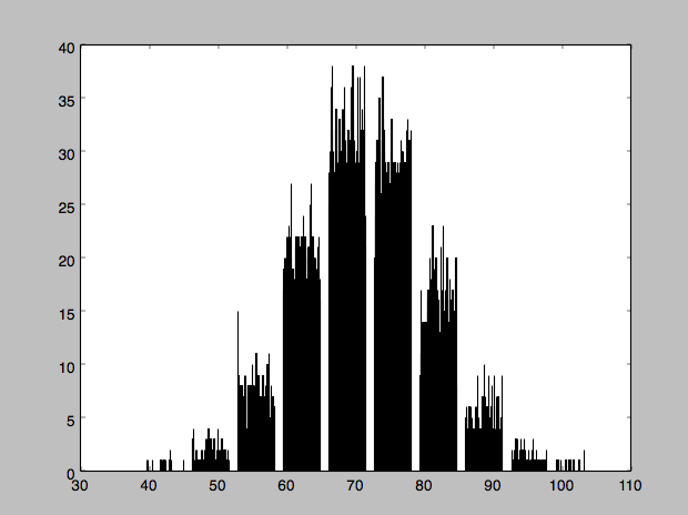
That’s a bit undersampled, but not insane. I noticed that you’re assuming a gain of unity by setting the variance to the mean of that lower-left corner, but that looks to be about right. A single pixel all around the image is systematically low, but that shouldn’t cause what you’re seeing with the deblender. There are pixels distributed over the image with a value ~ 100, where the sky is 71 +/- 9, so these are a bit over 3-sigma significant, but there are rather more of them than I would have expected. So I plotted a histogram and it looks rather weird:
>>> import lsst.afw.image as afwImage
>>> image = afwImage.ImageF("scene.fits[Z]")
>>> pyplot.hist(image.getArray()[1:100,1:100])
I’m gonna suggest that the strange statistics in your image are causing the extra peaks. I would strongly suggest you fix your images, but if you must use them then you could try tweaking the detection threshold in the SourceDetectionTask's config.
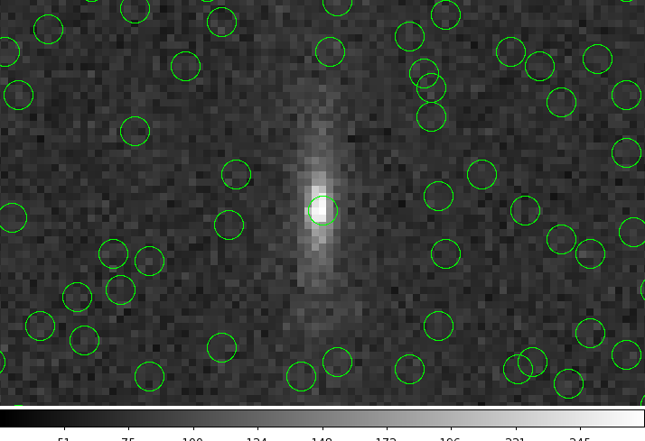
Plotting the source positions (which are coming from peaks in the convolved image), I don’t see anything in the extra peaks. It looks like the detection threshold is somehow crazy low.
Oh, here’s an idea — the background isn’t subtracted in your image. I wonder if our background subtraction (which I think should be running as part of SourceDetectionTask) is failing because the image is small. In any case, if you subtract the background before running detection, you should be better off.
>>> import lsst.afw.image as afwImage
>>> import lsst.afw.table as afwTable
>>> import lsst.afw.display.ds9 as ds9
>>> image = afwImage.ImageF("scene.fits[Z]")
>>> catalog = afwTable.SourceCatalog.readFits("stack_catalog.fits")
>>> ds9.mtv(image, frame=1)
>>> with ds9.Buffering():
...  for src in catalog:
...   ds9.dot("o", src.getX(), src.getY(), frame=1)
...
Maybe this is wrong but when I do this “pseudo-background subtraction” I obtain only 7 sources (still not great but much better)
Here’s what I add to the code:
variance = (numpy.percentile(scene_hdul['Z'].data.flatten(),75)-numpy.percentile(scene_hdul['Z'].data.flatten(),25))*0.7413
bkg = numpy.mean(scene_hdul['Z'].data[0:50,0:50])
print variance, bkg
deblend_run(
    image_array=scene_hdul['Z'].data-bkg,
    variance_array=variance * numpy.ones_like(scene_hdul['Z'].data),
    psf_array=psf_hdul['Z'].data,
)
And if that doesn’t work, try using the debugging outputs. Put a file called debug.py on your PYTHONPATH, with the following contents:
import lsstDebug
print "Importing debug settings..."
def DebugInfo(name):
    di = lsstDebug.getInfo(name)
    if name == "lsst.meas.algorithms.detection":
        di.display = 1

    return di
lsstDebug.Info = DebugInfo
Make sure you’ve got display_ds9 setup, and add import debug to your script.
Thanks for the suggestions @price and @fjaviersanchez! Based on this output, I think it is trying to subtract the background:
sourceDetection: Detected 1 positive sources to 5 sigma.
sourceDetection: Resubtracting the background after object detection
But I will try pre-subtracting. I believe there is a way to disable background subtraction (perhaps I saw it in the obs_file code?) so I will try that in conjunction with pre-subtracting the sky level.
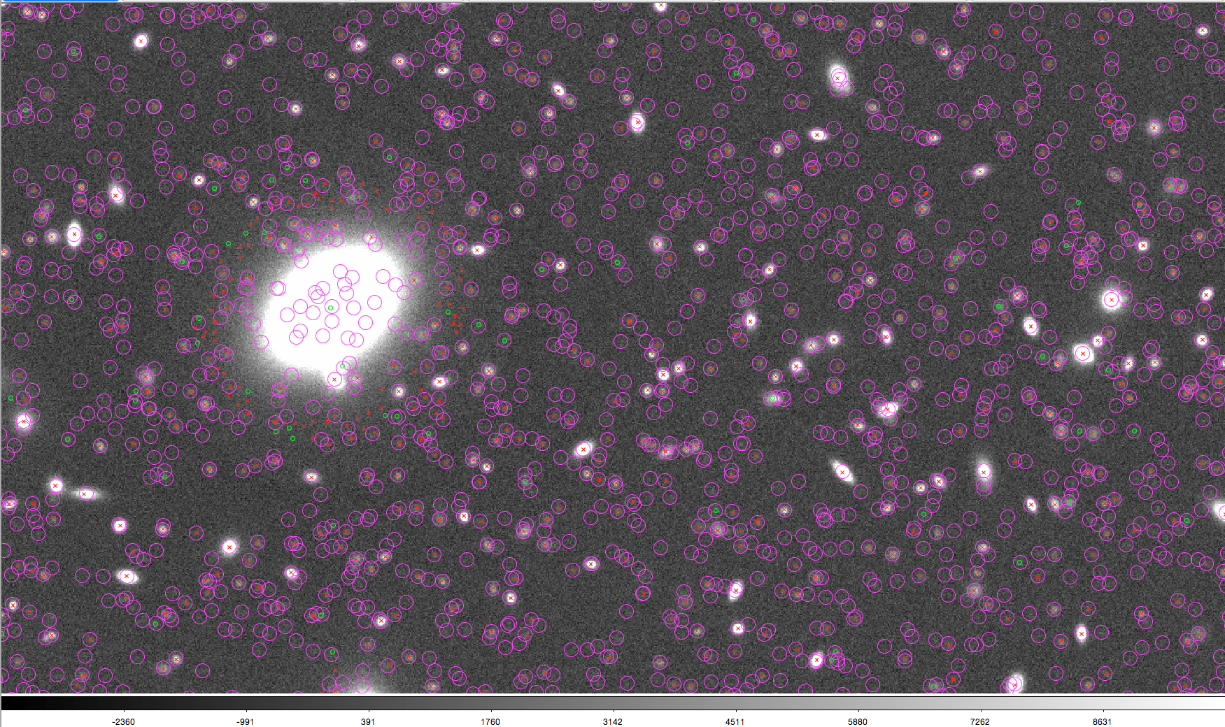
I have some results from running the stack on simulated images.
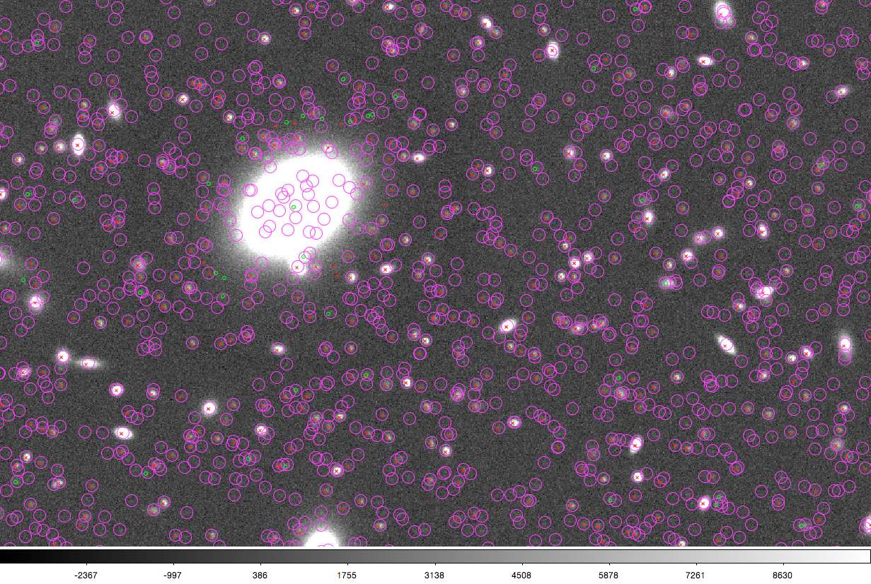
In the first image I compare the simulated inputs (magenta circles) with the detections from the stack (red crosshairs and green circles). The green circles are sources where sdss_baseFlux=NaN
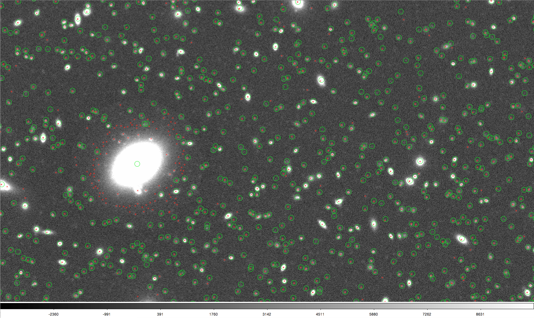
This second image compares the output from SExtractor (green circles) and the stack (red crosshairs).
There are some spurious detections around the brightest galaxy, I think it’s because the flux of the bright galaxy is not subtracted properly and generates these objects. These images are simulations up to LSST full-depth.
It’s actually because the background subtraction is too good, so that noise in the wings of the galaxy causes peaks to be detected. The solution/workaround is to over-subtract the wings of the galaxy (subtracting the background with a smaller spatial scale), which is what the SourceDetectionConfig parameter doTempLocalBackground enables; set it to True. You might have to tweak tempLocalBackground.binSize; it defaults to 64 pixels.
I was playing around with this, and I’m not sure I understand what is strange here… If you use plt.hist(image.getArray()[1:100,1:100].flatten()), you should see a normal distribution about the sky level (~71 counts per pixel). This is what I expect to get out from the noise I’m adding in.
import lsst.afw.image as afwImage
image = afwImage.ImageF("scene.fits[Z]")

plt.figure(figsize=(12, 4))
plt.subplot(121)
_ = plt.hist(image.getArray()[1:100,1:100].flatten())
plt.xlabel('counts')
plt.ylabel('N pixels')
plt.subplot(122)
plt.imshow(image.getArray()[1:100,1:100], cmap='gray')
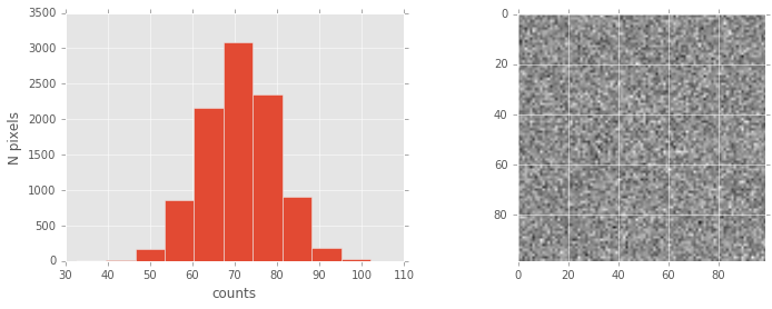
This distribution is slightly lopsided towards the high-count pixels because of (I believe) the edge of the galaxy profile extending into the sky estimation box. Is there something else wrong with this picture that I’m missing? (I’m not an expert in making realistically noisy scenes!)
Sorry, I screwed up — neglected the flatten(). No idea what matplotlib was plotting.
Ah, well at least it’s not something wrong with the image! I guess that puts me back where I started, with the bogus detections. It looks like background estimation and the detection threshold are set correctly for the sourceDetection step, but perhaps sourceDeblend isn’t getting the message? I can only speculate since I don’t know if that would explain what we see.
I did try to pre-subtract the background level by averaging a box from the corner and subtracting that average off image_array. I also tried lsst.afw.math.makeStatistics(image, lsst.afw.math.VARIANCECLIP).getValue() which gave a similar number.
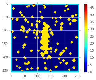
Pre-subtracting the background and supplying detect.config.reEstimateBackground = False gives a mask image that’s a little more interesting to look at, but still not what I would expect:
So, having looked at the code, SourceDetectionTask doesn’t do an initial background subtraction. You need to give it a background-subtracted image.
I ran your code (after a few tweaks: background subtraction, fix use of SourceDeblendTask; I’m running with the recent weekly, w_2016_32) and got what looks like a respectable number of sources:
pprice@tiger-sumire:~/temp/josePhoenix $ python test.py
sourceDetection: Detected 1 positive sources to 5 sigma.
sourceDetection: Resubtracting the background after object detection
sourceDeblend: Deblending 1 sources
sourceDeblend: Deblended: of 1 sources, 1 were deblended, creating 4 children, total 5 sources
measurement: Measuring 5 sources (1 parents, 4 children)
measurement WARNING: Error in base_SkyCoord.measure on record 2: Wcs not attached to exposure.  Required for base_SkyCoord algorithm
measurement WARNING: Error in base_SkyCoord.measure on record 3: Wcs not attached to exposure.  Required for base_SkyCoord algorithm
measurement WARNING: Error in base_SkyCoord.measure on record 4: Wcs not attached to exposure.  Required for base_SkyCoord algorithm
measurement WARNING: Error in base_SkyCoord.measure on record 5: Wcs not attached to exposure.  Required for base_SkyCoord algorithm
measurement WARNING: Error in base_SkyCoord.measure on record 1: Wcs not attached to exposure.  Required for base_SkyCoord algorithm
Thanks @price! Changing tempLocalBackground.binSize helped a lot. I used 8, 16, and 32 pixels and the results improved significantly. I am still getting some spurious detections but it behaves much better. This plot shows the results with tempLocalBackground.binSize=8. Red crosshairs are sources detected by the stack and with base_SdssShape_flux != NaN. Green circles are sources detected by the stack but with base_SdssShape_flux = NaN. Magenta circles show the simulated sources.
How should base_SdssShape_flux = NaN be interpreted?
The SDSS shape measurement has trouble at low S/N (the adaptive moment is probably diverging), so I think you can generally interpret a NaN flux as “this thing is faint”. I’ve never used base_SdssShape_flux for science; there are much better measures. In particular the base_PsfFlux_flux should have a fairly sharp cut-off (because we’re using the PSF for detection) and yet be well-behaved at the faint end, so that’s usually what I use for my ordinate when plotting.
Is there an easy way to get the individual postage stamps from the deblended objects?
Have a look at meas_deblender/examples/plotDeblendFamilies.py
So when I compare the input centroids to the recovered centroids (either sdssShape, naiveCentroid, GaussianCentroid or HSMSourceMoments) I get a systematic trend for the recovered centroids to be lower in both X and Y axes (so the centroids are displaced down and to the left). At the beginning I thought it could be due to some sort of alignment in non-detected blended sources but, I changed the field and it still happens the same. I made sure that the PSF is centered in the central pixel (it’s 75 x 75 pixels and the maximum lies at [37,37]). Are there any tunable parameters to change the centroid estimation? Any ideas of what I could be doing wrong?
Green ‘+’ are the input centroids and black ‘x’ the recovered centroids.
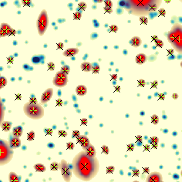
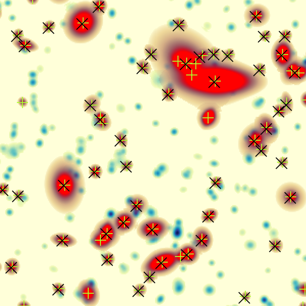
LSST centroids are zero-indexed (lower-left corner is 0,0) rather than following the FITS convention of unit-indexed (lower-left corner is 1,1).