It is mid-July and as mentioned in the June 2019 update, we have some new runs for you.
Book keeping:
This set of runs are labelled as “FBS 1.2”, while the previous set (June 2019 and prior) will be labelled “FBS 1.1”. In each version, we will re-run all of the previous still-relevant runs (so, at this point, all of them). This will make sure that we are comparing apples-to-apples when making comparisons between rolling cadence runs or various footprints, for example. However - at this point, we are NOT changing the names of the runs!
The version information is preserved inside the output database, in the “info” table, and is clearly labelled in the online MAF tables. At this point we’re only keeping the up-to-date runs online. Please let us know if this is going to create a problem for you – while we hope this will make it easier to keep straight which run is which within a set (instead of having runs identified simply with numbers), having the same names also adds a bit more burden on your end to make sure you have “baseline10yrs” from FBS 1.2 or FBS 1.1. At this point, I’d anticipate a set of FBS 1.3 runs in mid or end of August (hopefully before PCW, but likely not), and then we would likely have new releases of runs every two months or so.
FBS 1.2 runs
On to the fun stuff. The links below for this set of mid-July FBS 1.2 runs are to the databases at https://lsst-web.ncsa.illinois.edu/sim-data/sims_featureScheduler_runs/
They are also available at http://astro-lsst-01.astro.washington.edu:8081 – we will work on adding to the MAF outputs at that location. The MAF outputs are identified by the same run names as the DB links.
FBS 1.2 runs include:
-
baselines Variations on the baseline intra-night visits - comparing 1x30s vs. 2x15s visits and comparing pairs in the same filter vs mixed filters (or even no pairs). For other sets of simulations, we have taken the 1x30s + mixed pairs of filters example as the standard intranight cadence … however please take this as a working premise, but not an official constraint or choice. My understanding is that the final decision to choose 1x30s vs. 2x15s visits will not be made until on-sky observations with the survey camera are aquired.
- no pairs
- pairs in the same filter
- pairs in mixed filters
- pairs in the same filter, 2x15s visits
- pairs in mixed filters, 2x15s visits
- here’s the directory containing the databases for these runs – hopefully the naming scheme is becoming more clear? [roughly … some modification of category + identification of run feature].
-
footprints Limited variations on the WFD footprint. Takeaways from these simulations should include: how is extragalactic science benefitted from the variation in the WFD footprint (the primary driver for going to 18,000 sq deg with low galactic extinction)? How do the changes in the WFD footprint impact other science? For now, we’ve taken the ‘traditional WFD’ footprint to be the basis for most of the other experiments, but this will may change in a future set of simulations.
- baseline … equivalent to baseline_1exp_pairsmix_10yrs above, and following the traditional baseline footprint for WFD
- gp_heavy continue traditional WFD coverage throughout the galactic plane (low galactic latitude regions + bulge)
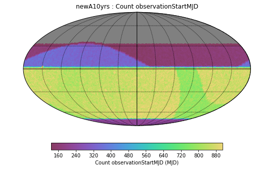
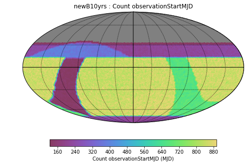
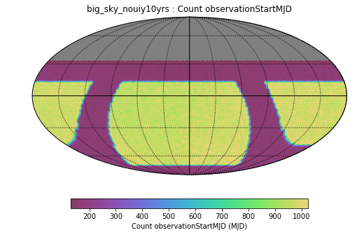
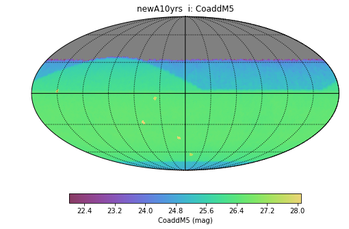
- big sky a footprint roughly matching that suggested by the “Big sky” whitepaper - extends WFD north (+12) and south (-72), limited by |b|<15 from low galactic latitude regions.
- Some further interesting variations on these extended N/S WFD regions, playing on different hypothetical/placeholder minisurvey configurations. Some of these limit the WFD region to 825 visits, versus 90% of all visits. The rest of these runs are available here. Here is a visualization of these footprints.
- To do: cover WFD with only 825 visits per healpix, vs. cover WFD with 90% of total visits. Define low galactic latitude limits more precisely than |b|<15 (instead, by E(B-V)<0.15) and run simulations using this limit. Run simulation of extended N/S WFD with ‘traditional’ diamond-shape galactic plane region.
-
Rolling cadence A range of variations on the rolling cadence. There is more to do here, but we need better metrics to distinguish between the effects of these difference cadences. The rolling cadences tested so far are all declination band-based. Then, in general, there are two categories: a ‘simple’ version where the cutoff for changing between dec bands is a single time for all points on the sky (so seasons at some points in the sky can be split), and a ‘modified’ version where the time for changing between dec bands depends on RA (so seasons are always contiguous). The modified version requires waiting a little longer before starting and after ending the rolling period. For each, there are variations on the number of dec bands: 2, 3, 5, and 10 for the ‘simple’ version, and 2, 3 and 6 bands for the ‘modified’ version. For the ‘modified’ runs, there are also variations on the weight for the ‘background’ (non-rolling / non-emphasized) portions of the WFD, from 5-20%. For the ‘simple’ runs, the background WFD is carried at 20% of normal weight. In each run, the intranight visits are in mixed filter pairs. For now, we’ve taken a non-rolling cadence as the basis for other experiments, but this may change in a future set of simulations.
- Modified rolling, 2 bands, 5% background WFD
- Modified rolling, 2 bands, 10% background WFD
- Modified rolling, 2 bands, 20% background WFD
- Modified rolling 3 bands, 5% background WFD
- Modified rolling 3 bands, 10% background WFD
- Modified rolling 3 bands, 20% background WFD
- Modified rolling 6 bands, 5% background WFD
- Modified rolling 6 bands, 10% background WFD
- Modified rolling 6 bands, 20% background WFD
- Simple rolling 2 bands, 20% background WFD
- Simple rolling 3 bands, 20% background WFD
- Simple rolling 5 bands, 20% background WFD
- Simple rolling 10 bands, 20% background WFD
-
DDF Limited variations on the DD sequences we simulate. Most of these have been targeted at simple questions regarding how to dither the DD fields, but a DD simulation matching the DESC requested DD cadence is available. For now, we are using a ‘traditional’ non-dithered DD sequence for other simulations, but this is likely to change in future simulations.
- DD DESC cadence
- DD directory The other runs are variations on the dither strategy - some with a large translational dither (0.7 deg) and some with a small translational dither (0.23 deg), and some only dithering once per night (‘pn’) and some randomly for each observation.
- To do: create simulations with AGN requested DD sequences, and create runs shifting our current (somewhat random) 5th DD field location to the suggested Akari field location.
-
ToO Experiments to add ToO sample observations, at a varying rate of triggers. In each, the ToO requested observations themselves are similar; a circular region of sky with a 15deg radius (so about 700 sq deg per alert) is covered in each of g, r and i bands 3 times (9 observations per location in the alert area) within 3 days of an alert being issued. The rate of alerts is varied in each simulation, from 1 per year to 100 per year. The takeaway here would include looking at the impact on other science, and how these impacts compare to other downtime.
- 1 ToO per year
- 10 ToO per year
- 50 ToO per year
- 100 ToO per year
- To do: make the ToOs themselves match the requested style of ToO’s from the white papers (or any updates from the PCW).
- Presto-Color The Presto-Color white paper requested triplets of observations in at least a subset of WFD fields, with more widely spaced observations in more specific colors (such as taking visits in a sequence of g - i - - g). We have some simple experiments with this cadence.
- Short exposures There were white paper requests for very short (1s or 5s) exposures over the entire sky in each filter. We ran simulations adding these mini-surveys, taking either 1s or 5s exposures 2 or 5 times per year.
-
altSched A series of simulations attempting to come closer to recreating the alt scheduler outputs, without some of the drawbacks to the alt scheduler. The alt scheduler schedules without consideration of lunar phase or weather conditions, which we would like to account for, and is based on a particular survey footprint. The benefits to the alt scheduler cadence include the more rapid inter-night revisit rate in given filters. In general, we’ve attempted to come closer to the alt scheduler by strongly weighting the region of ‘sky of choice’ for a particular night by dec region (to come closer to matching the per-night regions observed by the alt scheduler), and then looking at the effect of different weightings for features that affect filter choice.
- Heavy dec weighting - but more standard survey footprint, and maintaining standard features for filter choices (i.e. weighting m5 depths, etc.).
- Very_Alt - this incorporates the alt sched survey footprint more exactly, and forces y band into twilight, and tweaks the filter distributions.
- Very_Alt_rm5 - removes most of the m5 weighting per filter choice, to allow bluer filters to observe during bright time.
- Very_alt2 - attempting to spread filters (particularly z) throughout the month more, as part of a family that varies when the u and z/y band filters are swapped. See the series of these runs with ‘illum*’ variations on when the filters swap.
- Very_alt3 - similar to very_alt2, and again with a range of filter swap times, but now with increased weight on the m5 feature which should concentrate observations toward the meridian and shorter seasons.
- alt sched directory
-
Twilight survey Add a short exposure (1s) twilight survey, instead of taking standard visits during twilight. Basically this shows that the SRD requirements can be met without requiring twilight time.
- Twilight survey
- To do: run an NEO survey during twilight time, or other short-exposure twilight survey.
-
Rotator Weak lensing requirements suggest that a more uniform distribution of either rotTelPos or rotSkyPos would be desireable. This simulation is the first attempt to add rotator control into the simulator, and is worthwhile for understanding any effects of this control in general.
- rotator choose rotTelPos to make distribution more uniform
- Exposure Time Based on early feedback from the science collaborations, we had an early look at varying the exposure time to create visits with closer-to-uniform depth. We simply scaled the exposure time between 20s to 100s to maintain more uniform depth.
- Template generation Difference imaging will require a usable template image. This set of simulations experimented with adding weighting to parts of the sky which had not received a good image within the last ~250 days. The run parameters are similar, just with different weighting for this feature, the weight ranging from 1 to 5.
-
Filter changer The SAC recommended confining u band observations to within +/- 2 days of new moon, and understanding when to change the u band filter (for either z or y band) is useful. The takeaway from this set of runs is to understand the effects of changing the expected u band filter change time. We defined this based on lunar illumination - looking at 15, 30 and 60 % illumination.
- 15% illumination
- 30% illumination
- 60% illumination
- To do - write up the results of these experiments.
- Weather These runs varied the cloud cutoff point used to close the telescope, from 0.1 to 1.1 (representing the cutoff in amount of cloud reported by sims_cloudModel for any given time). Runs with 1.1 had no weather-related downtime and acquired 3.1M visits; runs with a cloud cutoff of 0.1 had the most weather-related downtime and only acquired 1.7M visits. See the comment about cloud cutoffs and weather downtime below.
-
Stability test These are primarily useful for tests of the sensitivity of the survey to details like the exact start date and random downtime. These are runs with changes to the start day of the survey, and changes to the random seed of the unscheduled downtime generation.
- Stability test directory
- To do; extend test to small tweaks to feature weights, make sure random downtime generation is working appropriately.
There is a lot to unpack there and we will be working on some more summaries of these runs before the PCW. In particular, looking at the general effects of the footprints and rolling cadences is high on our list, as well as the effects of the DD variations and filter options for pairs. We will have a short writeup regarding the filter swap timing soon, and I am also working on a writeup describing scheduling differences between opsim v3 and the new FBS (in particular, how the scheduler observes the sky on a given night).
Obvious items missing from the list of survey simulations above are mini-survey variations and galactic plane coverage variations, as well as a few more specific suggestions such as season extensions. These are still in the roadmap, but are not likely to be entirely complete before the PCW.
FBS 1.2 release notes
An important update taken in the FBS 1.2 runs is that we have increased our weather downtime significantly. Previous simulations had weather downtime on the order of 15%; comparison with SOAR and Gemini data indicate that this is within the range of downtimes, but is likely to be very optimistic.
Binned per-month, SOAR has downtime between 15% and 34%, while Gemini South provided a number of 915 downtime hours per year (about 30%). For this reason, we have decided to decrease the cloud cutoff in the cloud data we’re using, so that the survey downtime is about 32%, due to weather alone. This will overlap slightly with scheduled downtimes, but produces a notable decrease in the total number of visits expected. Please take this into account in your analysis!
The other important change is that the LSST throughput curves received an update to match as-measured curves for the lenses and CCD QE. This has improved the u band throughput, resulting in an increase in u band depth. We will note that there is a related bug we have found when calculating the total m5 depth per visit – currently the depth is always being calculated as if the visit was composed of 2x15s visits, even if it is a single 1x30s visit. This will be fixed in FBS 1.3 release, but it should be noted that the u and g band depths should be expected to increase slightly compared to the values reported in the FBS 1.2 runs as a result.