Discussion about science drivers for observations on Bulge and Crowded fields and development of static sky (very) crowded fields photometry pipeline
On February @ivezic addressed the SMWLV Science Collaboration (contact @jgizis for more info on this SC) and a few other experts on MW science asking to generate a list of well-motivated science drivers for observations in the bulge, plane, and Magellanic Clouds where the extreme crowdedness would not be well handled by the current LSST pipeline. LSST project is looking for science cases to appropriately direct resources to crowded field photometry pipeline construction. Note that the current tests indicate that the LSSt pipeline would perform well even on extremely crowded fields (200k start/deg^2) for transient science (i.e. the difference imaging pipeline adequately handles these fields) but the static sky photometry would not perform at this crowdedness limit.
This post is designed to continue the discussion, including asking questions on the content and format of the science-case documents that the Project has requested.
Is there a convenient standard map of the stellar source density for LSST on the sky?
(I feel like it’s a part of MAF but I’m not finding it right now. I’m not worried if the maps are based on an older model that could be off by factors of ~2.)
The maps in MAF (which are actually downloaded as part of the data from sims_maps, but read/used in MAF) are based on stellar density estimates derived from other simulations catalogs inputs, which in turn are derived from GalFast.
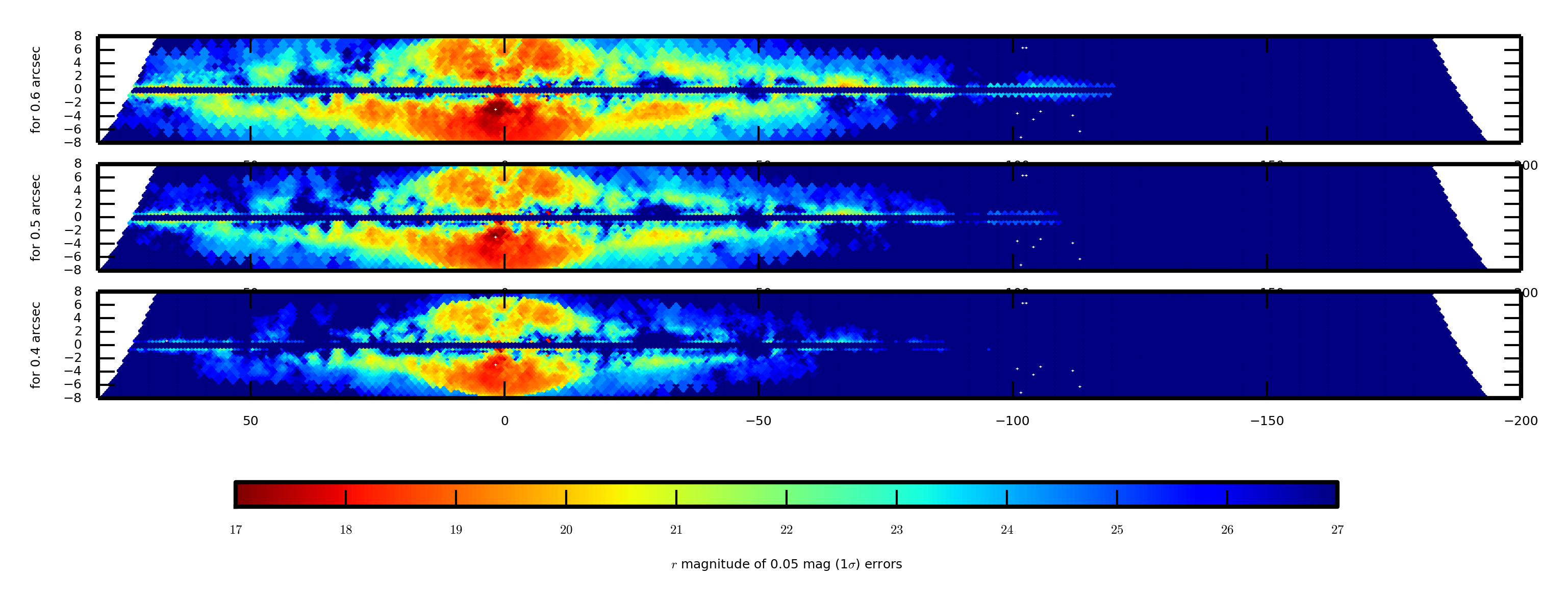
Our team has been preparing simulations alternative to GALFAST, which are partially uploaded to NOAO Data Lab (https://datalab.noao.edu/query.php?name=lsst_sim.simdr1) , but they are not yeat a good replacement to the maps in MAF mentioned above (especially because the DataLab files have big gaps in the Plane). Anyway, here are new estimates of the crowding limits in the r band, for seeing = 0.4, 0.5, 0.6, that is: these are the magnitudes at which photometric errors due to fainter sources will get larger that 0.1 mag. They agree with the DECAPS-based observation that the outer disk should not be crowded for LSST. Some areas in the inner Plane also appear as uncrowded, but simply because they have a huge extinction. Please contact me if you want to see some other related map – e.g. luminosity functions, distances we can reach for RC stars, etc.
@lgirardi these are great maps! Since you offered, could you please add:
expression you used for computing photometric errors due to fainter sources
similar maps that would give cumulative source counts per sq. deg. for sources
brighter than the crowding magnitude limit
for extra credit, integrated above counts within the Galactic plane diamond
(|b| < 10*(90-l)/90 for l<90 and symmetric for 270<l<360) would be super
useful, too.
Thanks!
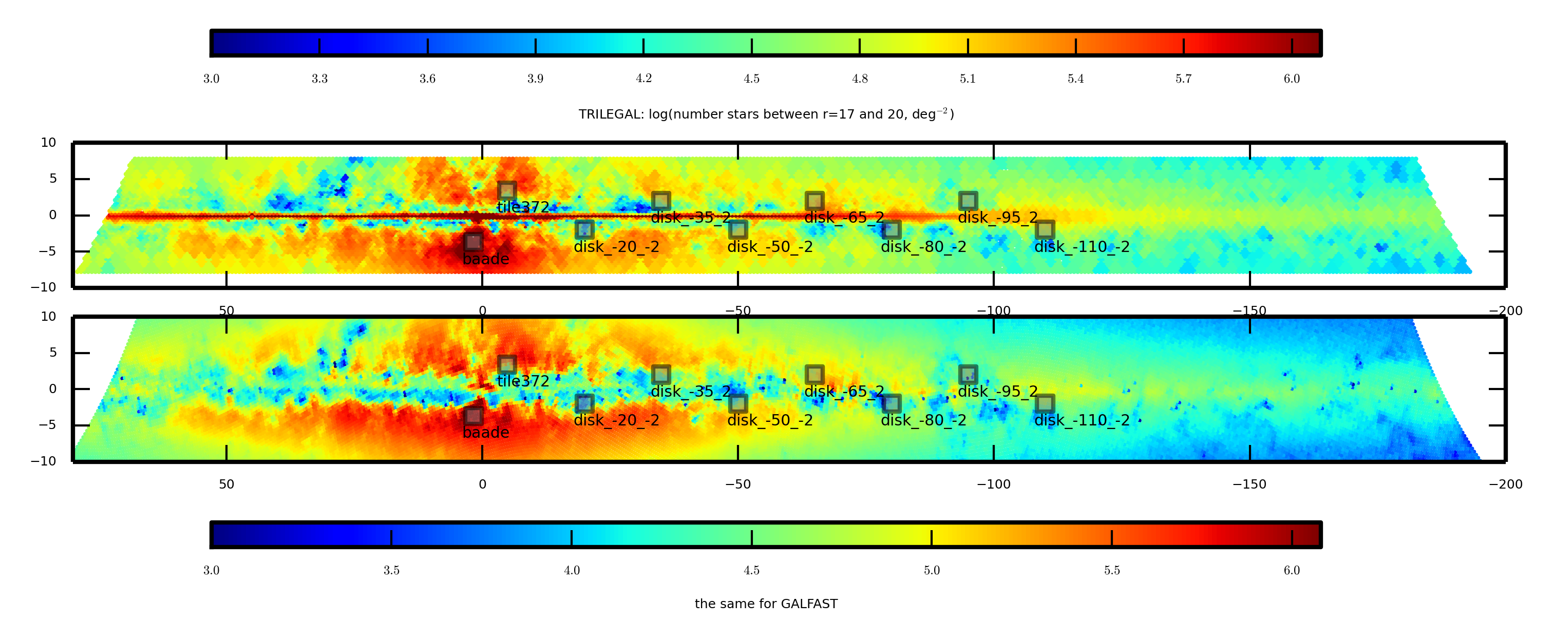
the density maps are below: that’s the log(Nstars/deg2) observable either above r=27.5, or above the crowding limit. There’s a weird effect that as the real stellar density increases towards the bulge, reaching the crowding limit suddenly causes the observable stellar density to decrease. Across the bulge and inner disk, for seeing=0.5 arcsec, we have a plateau with ~200000 stasr/deg2, similar to the limit you were mentioning for the current photometric pipeline! (if I got it right).
number of stars in the diamond area: (that’s a lower limit because the modeled area is somewhat smaller):
2.2e9 for seeing=0.6 arcsec
3.8e9 for seeing=0.5 arcsec
7.0e9 for seeing=0.4 arcsec
just a correction, in these maps, the crowding limit is considered to be reached at sigma=0.05 mag, not at 0.1 mag as I wrote in the previous post.
I have some preliminary estimate from the DECam Bulge data (the same as recently published in Saha et al. 2019, arXiv: 1902.05637v1). From a single DECam chip, at Galactic coordinates (0.84, -6.00), I have \approx 108k stars with in the i-band, in an area of 9x18 arcmin^2, that is a density of \approx 2.4 mln stars/degree^2.
The measured FWHM was 0.74 arcsec. The deepness was about i = 20.5, from the Saha’s paper.
This is only a daophot/allstar reduction (allframe usually goes deeper, because it adopts a forced photometry approach), and only stars with formal photometric uncertainties < 0.1 mag where selected.
The density is 1.8 mln stars/degree2 when only the stars with photometric error < 0.05mag are considered.
If you think this can be useful, I can proceed with a complete map.
To those using MAF to estimate stellar densities and magnitude limits: You might wonder if those numbers are realistic enough at low b. Here follow:
1- A reassuring comparison between stellar densities derived from GALFAST and TRILEGAL, at magnitudes 17<r<20, for which both simulations are complete. Apart the differences in the resolution and the strip of un-reddened stars that TRILEGAL has produced at b=0, one can say that two independent codes (calibrated on different data) produce something similar, roughly within factors of ~2 in stellar density.
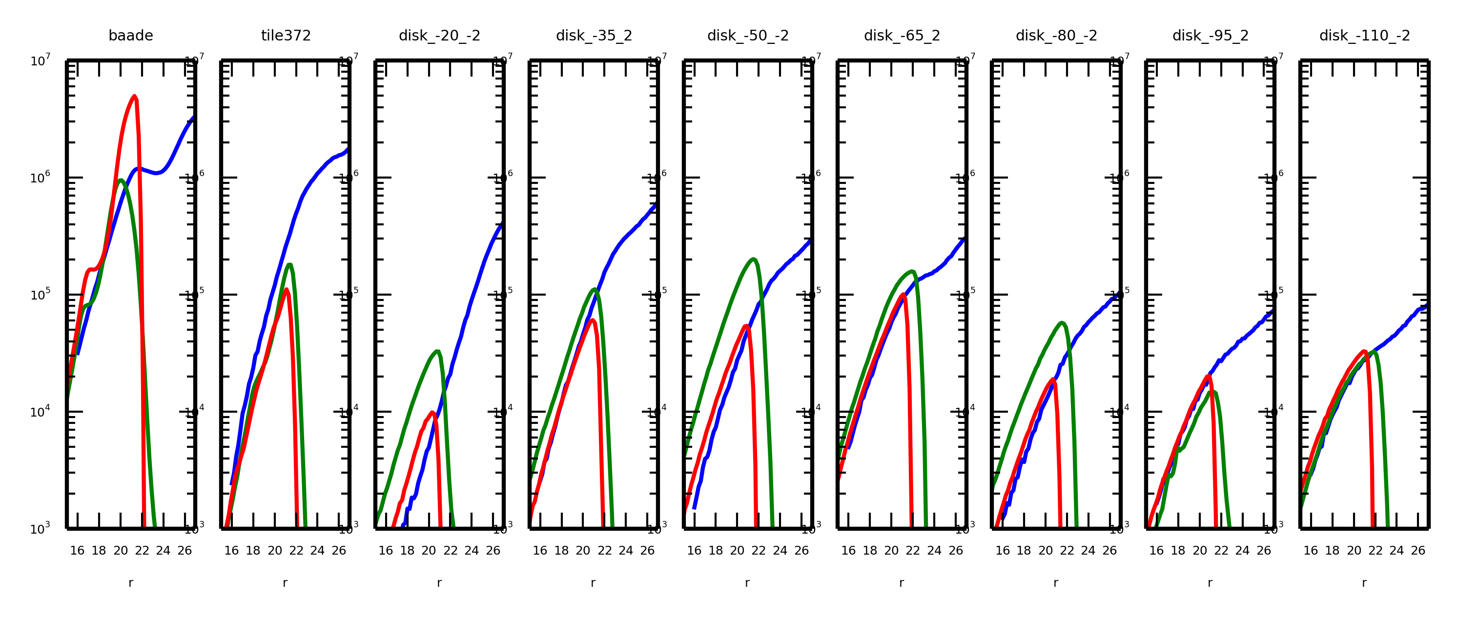
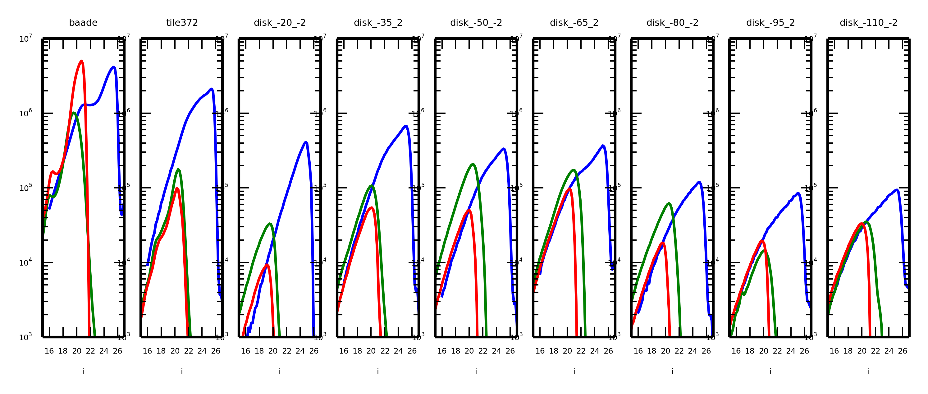
2- More importantly, here is a comparison with the real star counts from DECAPS, for selected low-b areas (thanks to Piero Dal Tio, Alessandro Mazzi, and Peter Yoachim for the help).
blue=GALFAST,
red=TRILEGAL (limited to g<23), and
green=DECAPS.
You can see that sometimes DECAPS star counts are largely in excess of the simulations, especially in highly extincted regions such as disk-20_-2 (Av from 6 to 11 mag) and disk_-50_-2 (Av from 5 to 9 mag). I interpret this as simply the result of putting the dust (from Schlegel or Planck maps) at too short a distance in the models.
Conclusions: MAF+GALFAST is good for discussing star counts for the moment, but we need better 3D dust models to improve its reliability close to the Plane. Of course one can use this as an argument for obtaining deep LSST star counts: they will improve 3D dust models at larger distances than DECAPS.
Please also look at the DECam data published by Saha et al. (2019, ApJ, 874, 30). The DECam field analyzed is at b ~ -4 (around the Baade’s reddening window) and about 1 million stars per degree^2 are found. More details in the paper.