I recently posted a Rubin Obs. technote, RTN-014: “Lunar Complications in the Scheduling of Deep Drilling Fields,” which raises some issues in scheduling DDF fields that I think science collaborations need to consider, particularly strategies for minimizing disruption in cadence by nights when the sky is bright enough that the limiting magnitude is several magnitudes brighter than nominal, or when the field is too close to the moon to be observed at all. I encourage anyone working on DDF strategy suggestions to take a look.
To further pique your interest (because this is cool work and has some implications for WFD scheduling/metrics too!):
When thinking about cadence, a simple approach is to just evaluate gaps between scheduled visits – these may be regular or may have longer intervals around new or full moon when filter availability changes (or just may occur due to needing to avoid observing too close to the moon).
In practice though, even if there are visits obtained near a full moon – those may not be useful visits for your science, due to changes in the limiting magnitude due to the moon!
When designing your metrics, you should consider not just the timing of visits but also the depth of visits compared to the magnitude of your desired sources.
Eric’s work here looks at how the changes in the limiting magnitude due to varying skybrightness would impose mandatory ‘gaps’ in coverage over the lunar cycle (assuming that the DDF sequences stay the same over the lunar cycle). Depending on the desired limiting magnitudes, DDF visits can be scheduled to minimize the resulting gap in coverage – but there are some complications, including the location of the DDFs on the sky. He suggests some of the options we can work on to incorporate more optimal scheduling of visits near bright time, and what some of those trade-offs may be. This is a really good place to start an in-depth discussion of subtleties with DDF cadences.
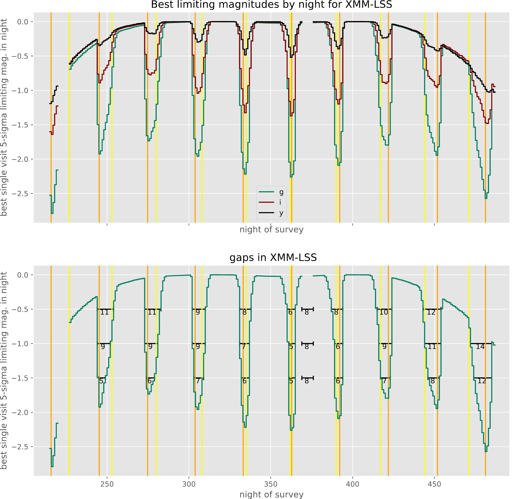
To illustrate: a nice plot from RTN-014 showing the ‘best’ limiting magnitude available in each night (assuming the field is observed at the best airmass and and skybrightness available in the night) over a season. The orange and yellow lines indicate when the moon is full and when the moon is closest to the DDF (respectively); the bottom panels indicates the minimum ‘gap’ in coverage, for a variety of g-band limiting magnitudes, and how these change over the season.
1 Like
Lynne et al,
I would also like to remind the readers that, regardless of moon phase or location, the sky brightness in the red band z & y in particular are highly variable. A significant contributor is the variability in upper atmospheric airglow. Depending on the solar activity level these variation can rather large amplitudes. I will see if I can find something quantitative.
Good point! @yoachim this (rapid timescale) variability in z and particularly y band is not currently included in the skybrightness model for the simulations, is it?
The high variability in sky brightness was quite apparent in DES data. I didn’t discuss it in this note, because I don’t have any suggestions on changes to scheduling because of it: there isn’t a lot we can do about it. (If we were to adopt variable exposure times in reaction to predicted depth, we may want to include sky brightness as well as seeing in this calculation, but I think that’s a separate discussion.)
For an idea of the magnitude, here is a plot measured sky brightness in DES vs. modeled sky brightness. The model used is much simpler than the one we use for Rubin, but I still think most of the offset between model and measured is due to intrinsic variability (e.g. from variable airglow) rather than limitations in the model.
Black points are exposures in fully dark sky, blue in sky with moon, orange during twilight. The red line is a perfect model fit.
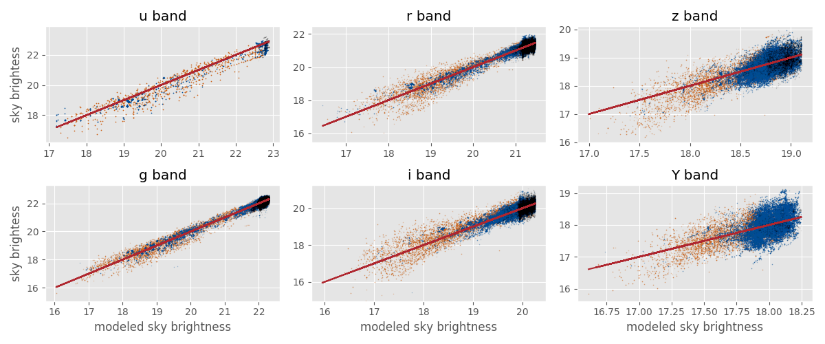
This plot and details of the DES sky brightness model are in appendix D of the DES scheduler tech note.
Numerically, the standard deviation of the residuals between DES model and measured varies from about 0.2 in bluer bands and 0.3 in redder ones.
The solar activity induced sky brightness changes are about 0.5 mags (full range). So taking the average value, our model will be off +/- 0.25 mags, and the resulting 5-sigma limiting depths will be off +/- 0.12 mags.
I’ve maintained we can mostly ignore the red filter variability because for values like final coadded depth the effect will average out. For the scheduler, the airglow is fairly gray, so it does little if anything to change where we would decide to point the telescope. If we’re in conditions where we would typically observe in y, and it turns out there’s lots of additional sky glow, it’s very unlikely we would be better off swapping to a bluer filter (z will also be brighter, and we were probably in y because the sky is bright in blue from the moon or twilight).
It seems like the way to go may be to just acknowledge there there may be a wider range of variability than is obvious in the simulations, and for the purposes of trying to schedule to avoid or metrics to calculate the expanse of ‘gaps’ we should try to consider the effect of this uncertainty.