A question from the Solar System science collaboration:
The summary file does not specify where the time is redistributed in the v2.0 DDF simulations. In the 3% DDF simulation, is the 2% extra survey time redistributed evenly between the areas within the Wide-Fast-Deep or to specific regions? In the 8% DDF simulation, is the extra 3% survey time now used by the DDFs taken evenly from the Wide-Fast-Deep or from specific regions?
Right! The DDF time is coming “off the top”, so when the DDF percentage is used, the rest of the time gets distributed to the rest of the footprint. The scheduler will try to maintain the same ratio of observations between different regions with whatever time is left. So increasing the DDF time will decrease the number of visits in all other regions somewhat evenly.
The simulations with 3% and 8% of survey time spent on the DDFs produce negligible (<5%) changes in our Solar System metrics, expect for the Jupiter Trojans. We find that the fraction of discovered Jupiter Trojans suffers for both increased (8% survey time) and decreased (3%) DDF observing time. We are uncertain as to whether this is because in the 3% DDF simulation the COSMOS field is being observed less, and in the 8% simulation time is taken away from the North Ecliptic Spur so less objects are observed.
Do you have any thoughts about what is causing this big swing in the Jupiter Trojans? They are very localized on the sky, but it was surprising to see that there was still an impact in both cases
That’s shot noise. It’s important to look at the raw values, not just the relative percent changes. For the v2.0 baseline, I get that DifferentialCompleteness H = 18.000000 Discovery_N_Chances Trojan 3 pairs in 15 nights trailing loss MoObjSlicer has a value of 0.0006. That means that out of the population of 5,000 Trojan orbits, 3 were detected. For similar but not identical simulations we should expect to detect 3 +/- 1.7 Trojans. I think those big swings are not statistically significant, we have a similar problem with the TDE metric a lot of the time.
Makes total sense. We hadn’t realized it was that few objects for the Jupiter Trojans that it could be Poisson small number statistics coming into place it was such small numbers detections. Makes a lot more sense now.
I believe these are cumulative completeness values, not differential completeness, though.
I apologize for the somewhat confusing name that these ended up getting in the summary stat CSV (I will update it appropriately). [the “short name” contains H<18, rather than H=18, and is correct]. @mschwamb if you want me to pull differential completeness out for these statistics instead, please let me know. We’ve done cumulative completeness instead for a while, for various reasons, but swapping could also make sense.
As cumulative completeness, the values reflect not just the completeness at H=18, but the completeness from the bright end down to H=18 weighted by something approximating the luminosity function - a power law with index alpha=-3.5.
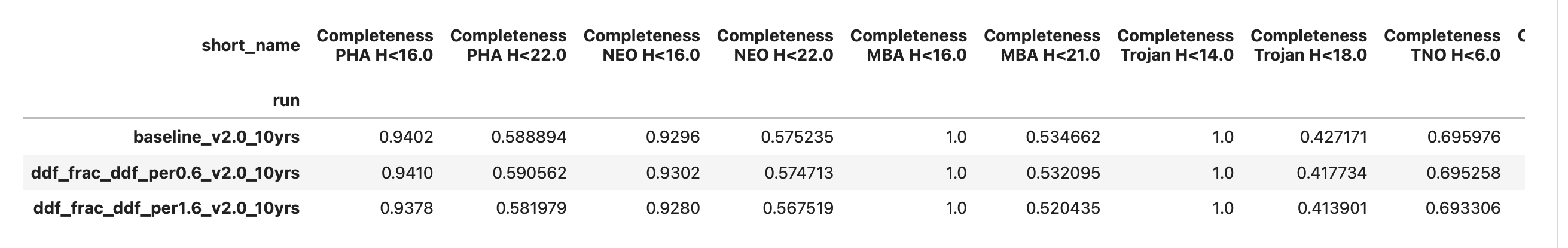
If you look at those raw numbers (see screenshot from the “Demo SSO metrics” notebook, which pulls in the CSV source containing the summary stats) the values are larger. That said, the swing due to the change in completeness of these smaller objects is still on the order of a %, which is only about 50 (out of 5000), and as @yoachim points out, the swing due to H=18 objects in particular is likely shot noise.
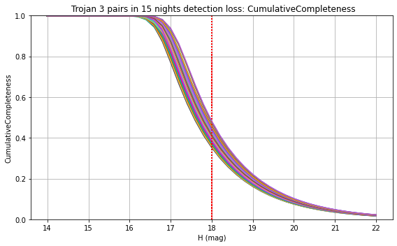
Plotting the full completeness curves for the Trojans across all simulations is pretty messy (thus picking out two points, one at the bright end and one approximately at the midpoint), but gives you an idea of the range of values:
The smoothness of all of these put together suggests to me that in some simulations, the completeness just starts falling sooner – which, together with the fairly steep drop-off, gives more dramatic results in the change of completeness at H<=18. It’s possible some of this is an artifact of using the same set of orbits and then varying the H value for the object over the range of interesting H values, but I don’t know if I expect that to be a big driver for the results. It’s also possible that the sharpness of the drop-off is actually varying more than Is visible from the (definitely very busy) plot.
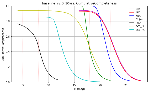
In general, I’ve felt that at the bright end, the biggest question is “does the survey cover the area that the objects reside in, in the sky”, because the bright objects tend to have lots of discovery opportunities because they don’t ‘disappear’ from many observations. At the fainter end, the question starts to become “were there enough observations in the survey that we could get good discovery opportunities” (perhaps the objects are not bright for very long – this is more important for NEOs or other more eccentric objects).
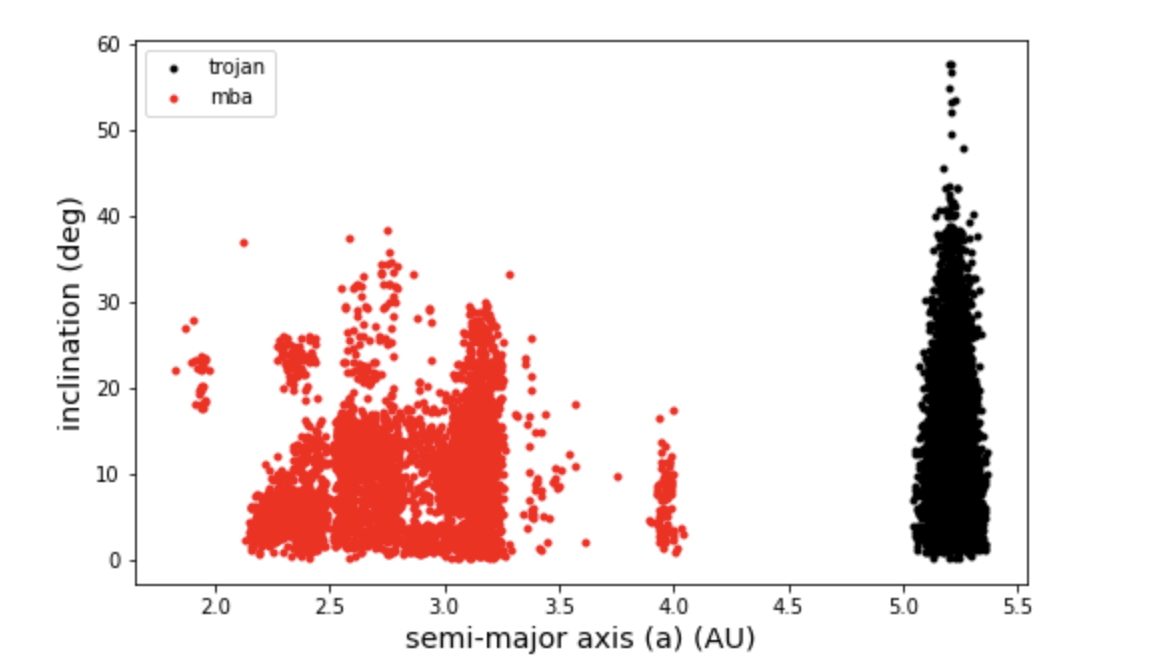
I’m not quite sure how this plays out for the Trojans, however. They have not-insignificant eccentricity, but it’s not more than the MBAs … on the other hand, they’re more limited in area on the sky, so perhaps this results in a stronger effect than otherwise expected? Maybe the biggest thing is that the Trojans cover a much more limited range of distances than other populations.
And looking at this plot below and noticing that the Trojans do seem to have the sharpest drop-off of any population, that this makes more sense as to why the faint Trojans show wider swings in completeness than any other population.