I have just finished what I’m hoping is a reasonable draft of our report to the SCOC and I made SO MANY PLOTS.
I think some of them are pretty cool, so I thought I might share some of them here as well. I know this looks like a lot … we should have conversations about them (maybe in separate threads).
But here we go.
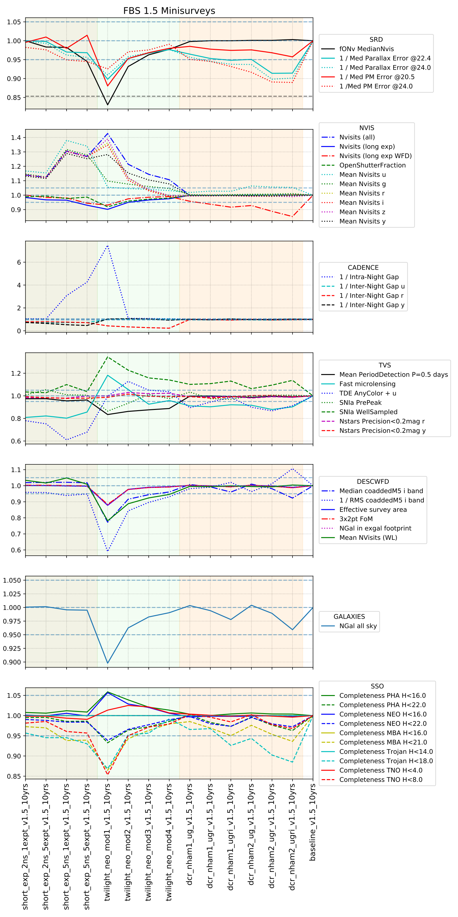
For each plot, I take a series of runs that I think deal with a related aspect of survey strategy, then take a series of different metrics (grouped by science, more or less. Each metric is normalized by a reference run from the set (usually the baseline run for that release), and values are inverted as necessary so that larger values should always be better.
For the SRD metrics, as there is a given value where things ‘fail’ for fONv Median Nvisits (i.e. this number can’t fall below 825), I add a dashed black line indicating where this failure point would happen.
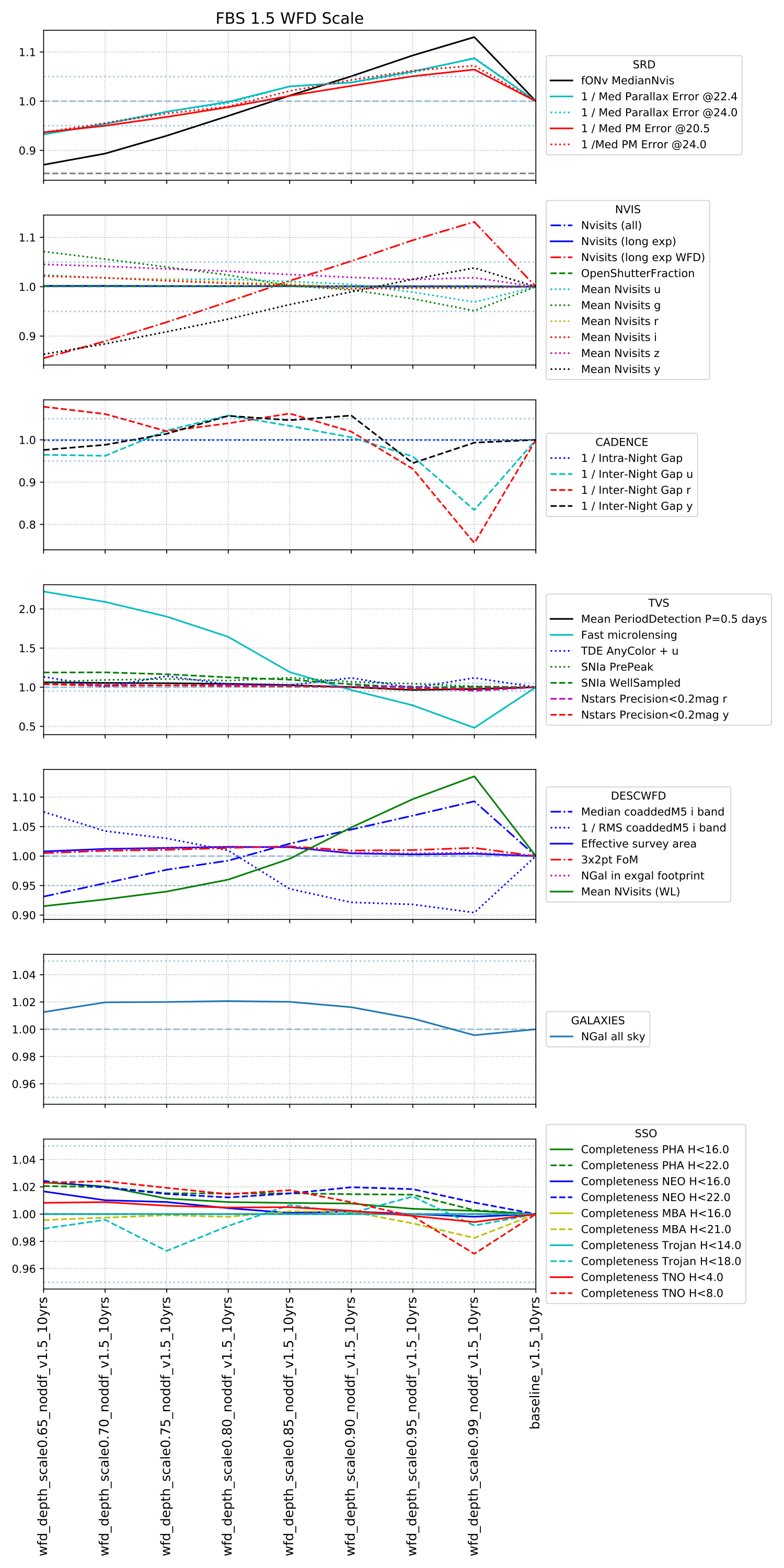
Why not start off with the family that simply scales the amount of time spent on the WFD? (wfd_depth_scale).
It is not surprising that the SRD metrics scale pretty directly with more time spent on WFD; after all, fONv tracks the number of visits per pointing over the best 18k square degrees (aka the ‘wfd’). It is also not surprising that as the fraction of time spent on the WFD approaches all the time (except for DDFs, which were held constant), that metrics for science which requires visits outside the standard WFD footprint start to crash.
To read this plot, note the names of the runs on the x-labels … these are the wfd_depth_scale runs, going from 65% time on WFD (left) to 99% time on WFD (right) … followed by the standard baseline run, which is the run the metric values were normalized against. Metrics which crash only at the highest fraction of WFD visits probably needed visits outside the WFD but managed to receive at least their minimum until that point. Metrics which scale from left to right are likely proportionally sensitive to the number of visits. Metrics which bounce up and down a bit may either be a bit noisy or may be sensitive to some aspect of the simulation variations that is not obvious (and if these were just statistical changes in the underlying simulation, it may still indicate a certain level of noisiness in the metric outputs).
A basic property of the survey is the visit exposure time. There are several options here – two snaps per visit (2x15s)[+], single snaps (1x30s), extending the u band exposure time to 60s to reduce readnoise issues[++], and/or adding variable exposure times to maintain more uniform individual image limiting magnitudes.
[+] This will remain the project baseline until the camera is on the telescope and taking data and we can confirm that 1x30s are a viable option, and even then, only after approving that change.
[++] The readnoise is more of an issue for u band because the sky is relatively dark in u. Occasional g band images are also readnoise limited, but typically this is primarily a u band issue.
It’s worth noting that the u60 simulation extends the u band visit time to 60s, but makes a corresponding reduction in the overall number of u band visits. This has a strong impact on transients which need u band visits for classification (this aspect is included in the TDE some color+u metric). To return the u band to the normal number of visits while maintaining the longer exposure time would require moving about 6% more of the WFD time into u band. This most likely would have to come from shifting visits in other filters into u (representing a shift of about 50-60 visits per field … a not insignificant change). Moving to fewer 60s visits does increase the final coadded depth in u band by 0.2 magnitudes.
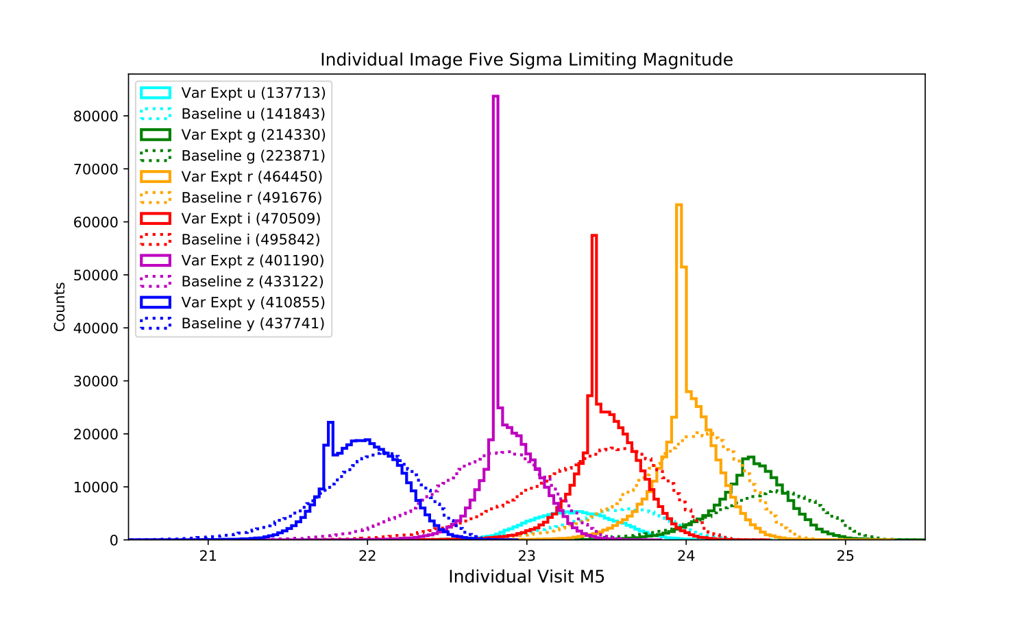
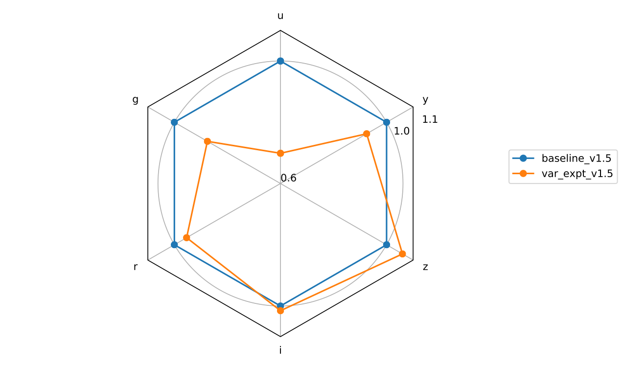
The variable exposure time simulation is interesting in that the individual image depths really do become more uniform – this might make it easier to track transients and variables over time. The overall on-sky time remained the same as well. Individual image times got slightly longer (mean of 32.2 instead of 30s). However, the final coadded depth in most bandpasses got slightly shallower; this is because most of the mean individual image depths are slightly shallower as well. This is something that could likely be tuned by parameters in the scheduler (changing the target single image depth), but it does add a lot of additional complications, including how this would apply with ‘live’ telemetry.
(histogram of individual image five sigma depths in the variable exposure run compared to the baseline 1x30s run)
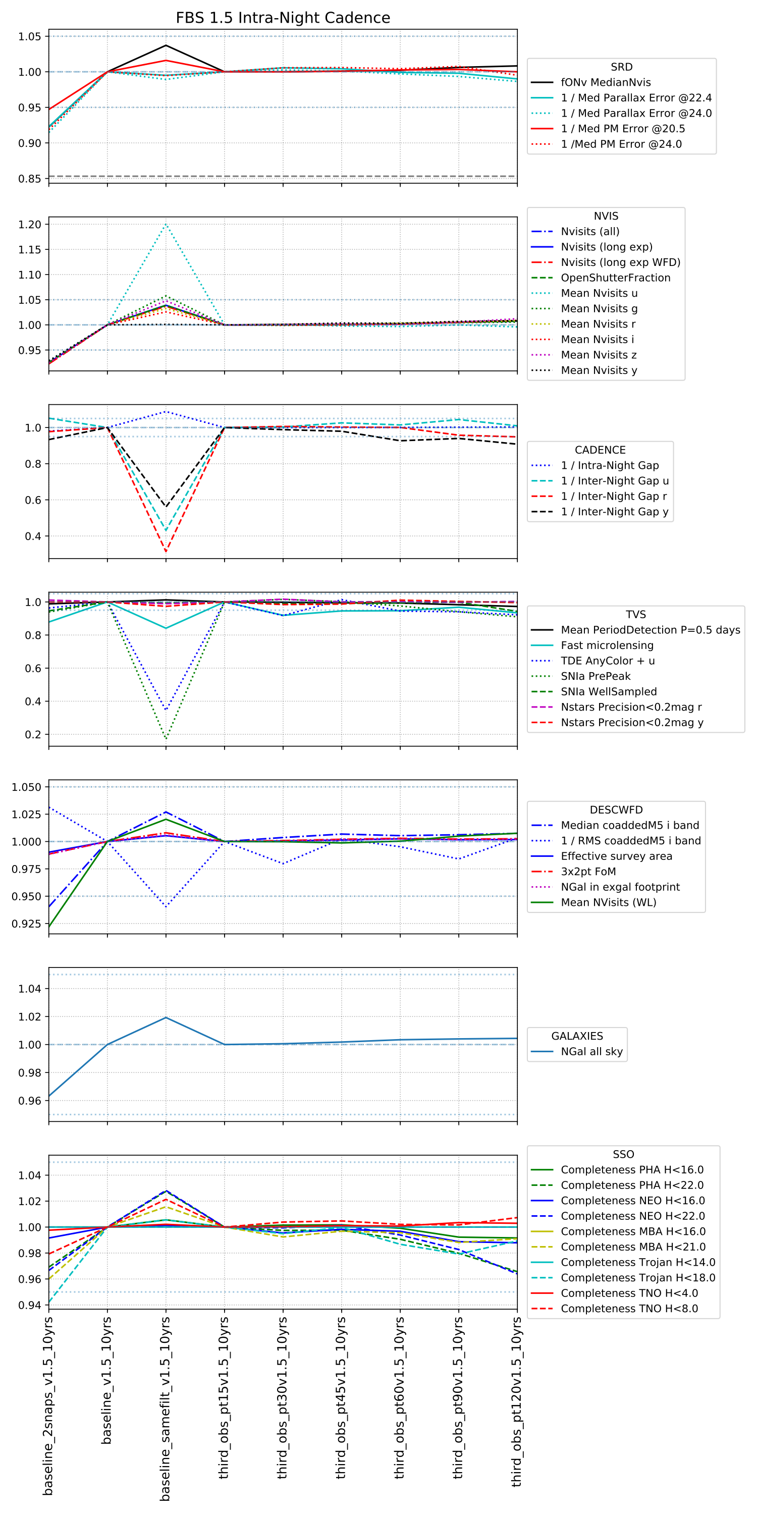
Intranight cadence – pairs within a night? in the same filter or different filters? what about triplets at the end of the night (with between 15 minutes to 120 minutes devoted to these triplets … the amount of time is reflected in the run name).
Pairs in the same filter are more efficient for observing (about 4% more visits overall). More visits is good for lots of science, and solar system science gets an extra boost beyond that because of the similar limiting magnitudes between pairs in this case (so not losing moving objects because you only see them in one visit). However transients and variables strongly prefer mixed filters.
Triplets, if they only take 15 to 45 minutes at the end of each night, don’t seem to have much impact. If the triplets are important for your science, I think we need your metric that shows how well these are helping.
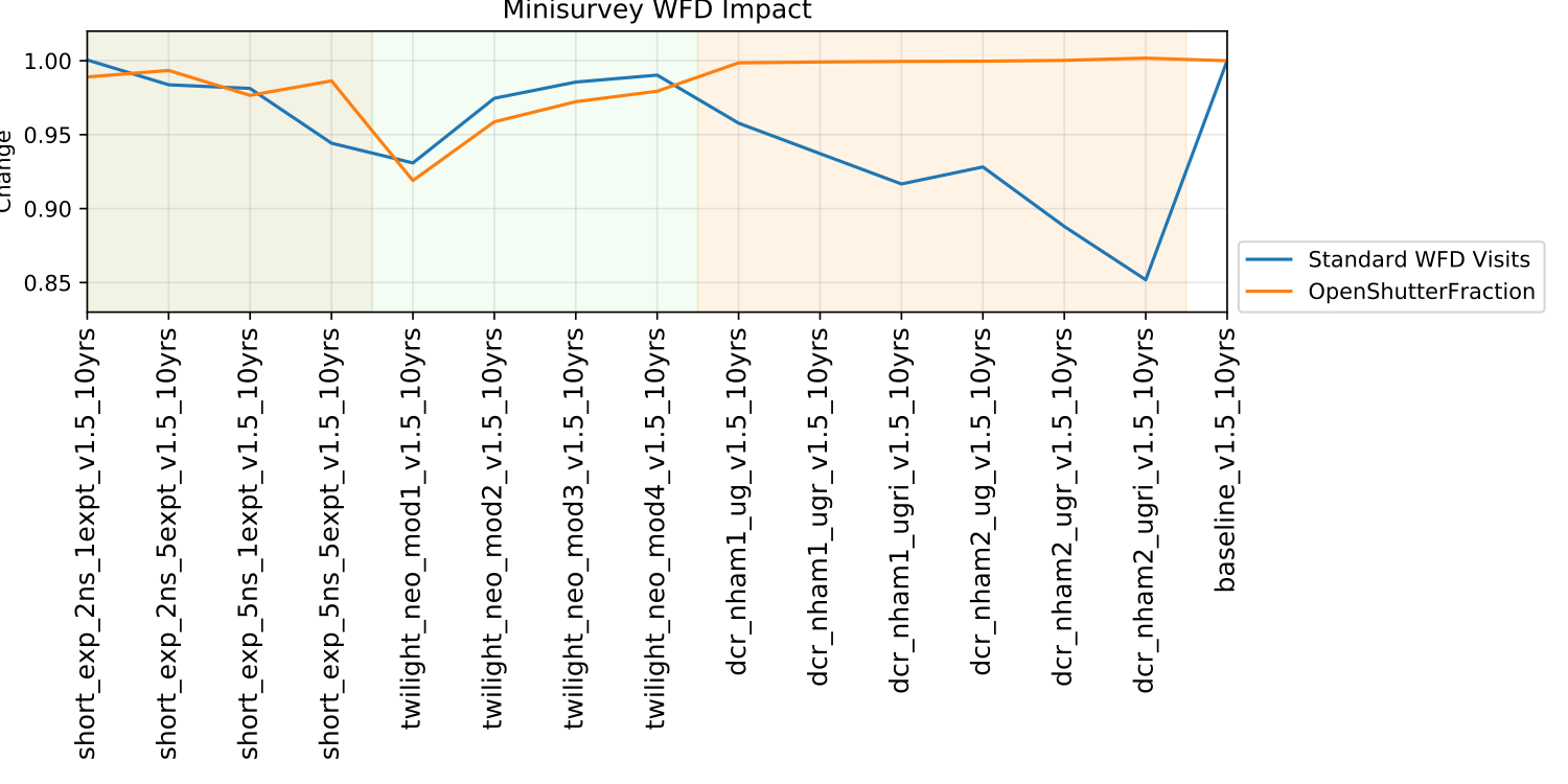
Minisurveys anyone? We tested minisurveys for DCR (getting high airmass visits), short exposures over the sky, and a twilight NEO survey. The impact on the main survey was variable, depending on how much the minisurvey observations could contribute towards the standard science metrics.
My takeaway from these is we need metrics that show how well each minisurvey is doing at the particular thing it was supposed to do (which we lack for the DCR and short exposure surveys, and could improve for the twilight NEO surveys).
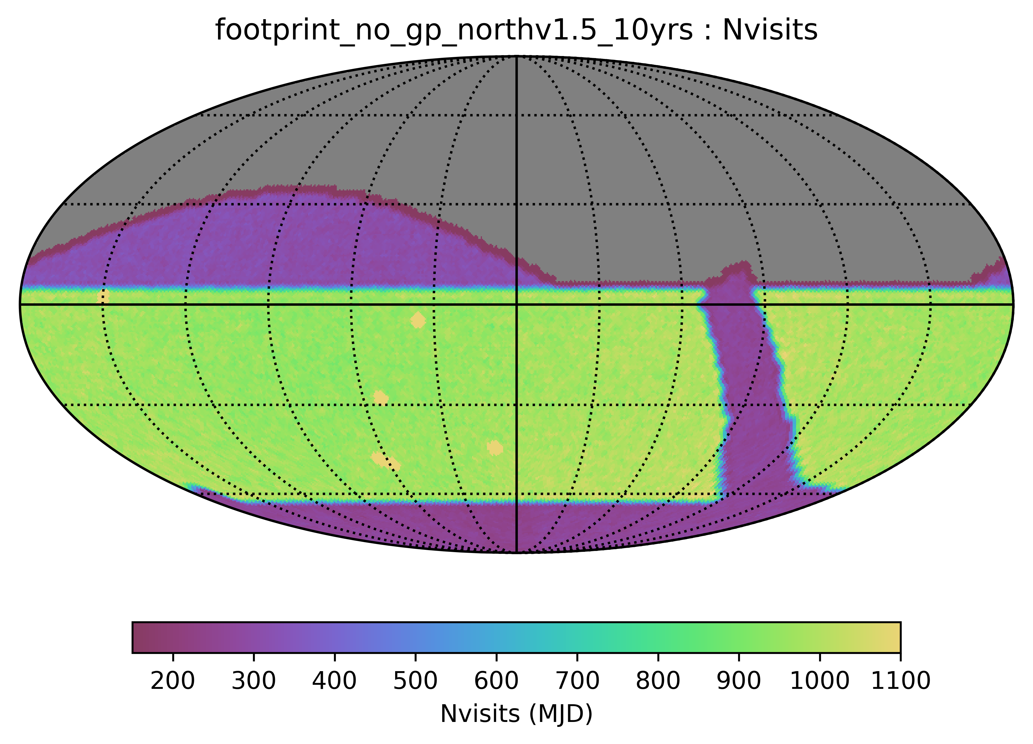
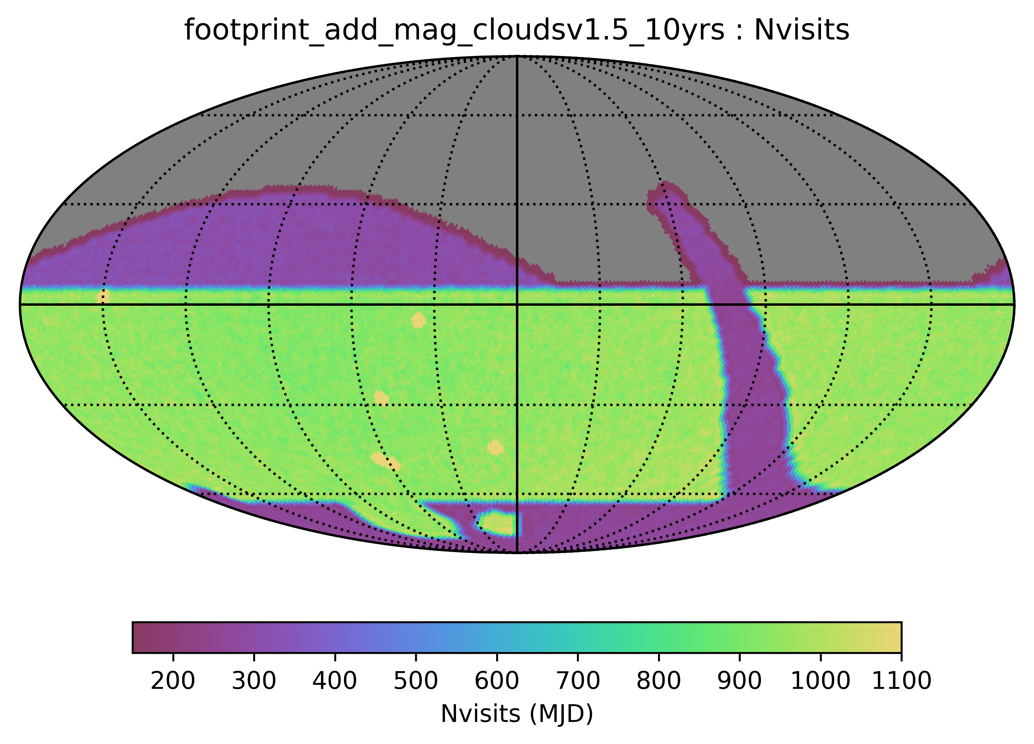
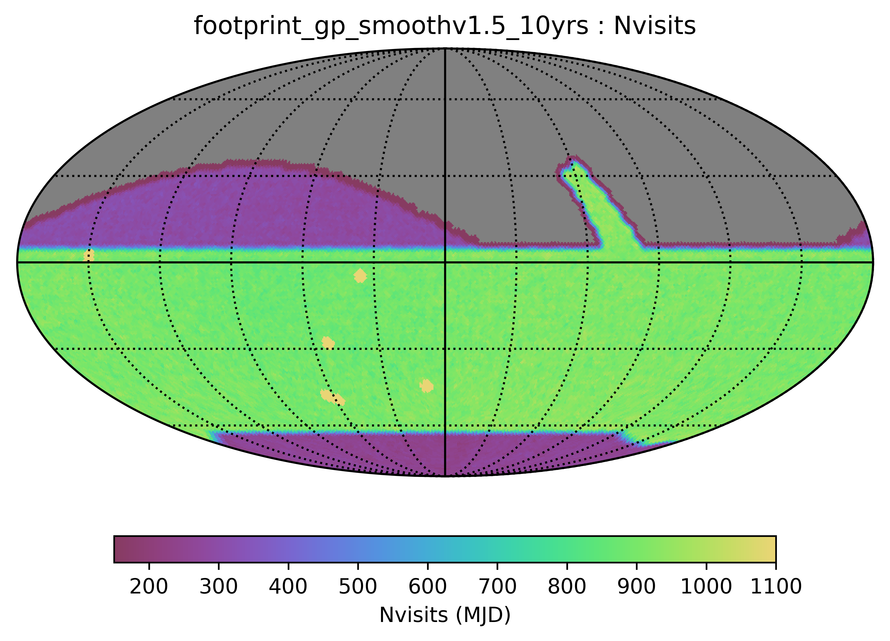
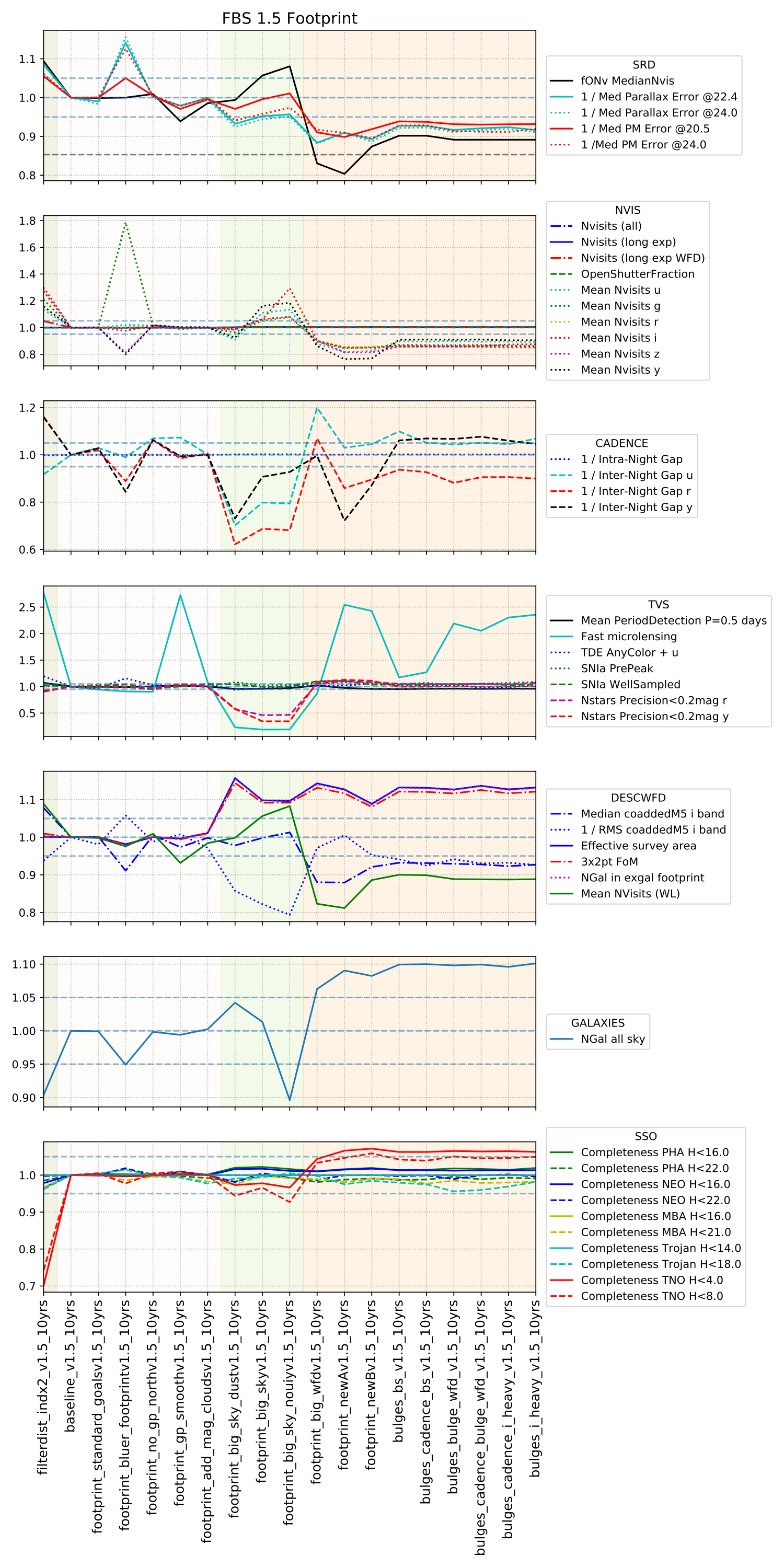
Some of the biggest questions revolve around the survey footprint. The survey footprints can be grouped into variations based on the current WFD region (-62 to 2 degrees dec, relatively small cutout around the galactic plane, includes high dust extinction regions) or variations based on a big sky WFD region (-72 to 12 degrees dec, larger cutout around the galactic plane, only low dust extinction regions). Variations on either footprint that don’t include the NES, SCP or GP have serious science drawbacks (see the ‘big_sky’, ‘big_sky_dust’, and ‘big_sky_nouiy’), so I look at this as we need to consider all of these regions at once. The ‘bulges’ simulations below include various levels of coverage of the galactic bulge.
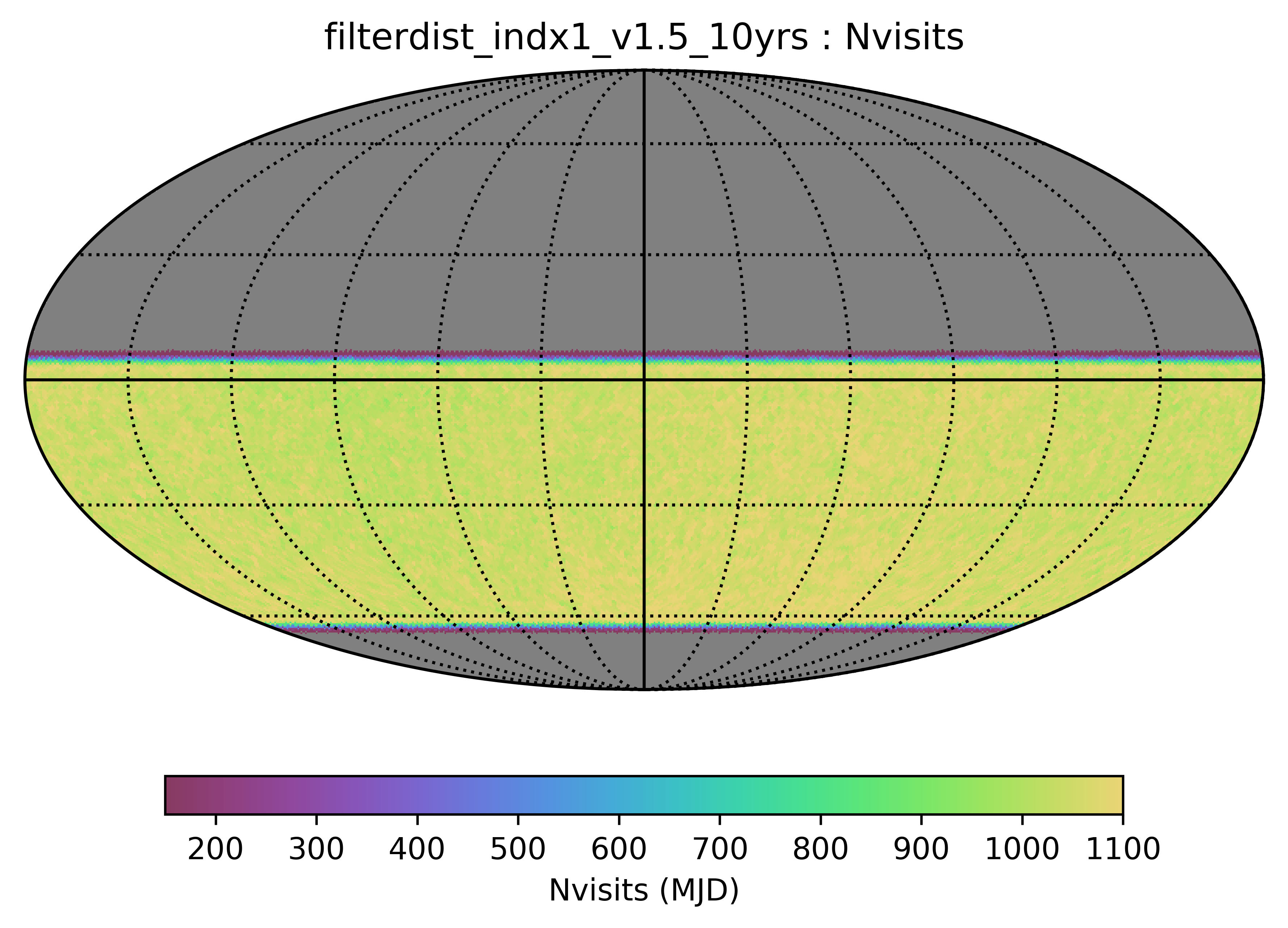
Limited WFD footprint types …
all of the filterdist runs have this same map, which covers a declination region similar to the standard survey WFD, with no variation across the galactic plane, and no NES or SCP coverage. The variations on filterdist have different filter distributions.
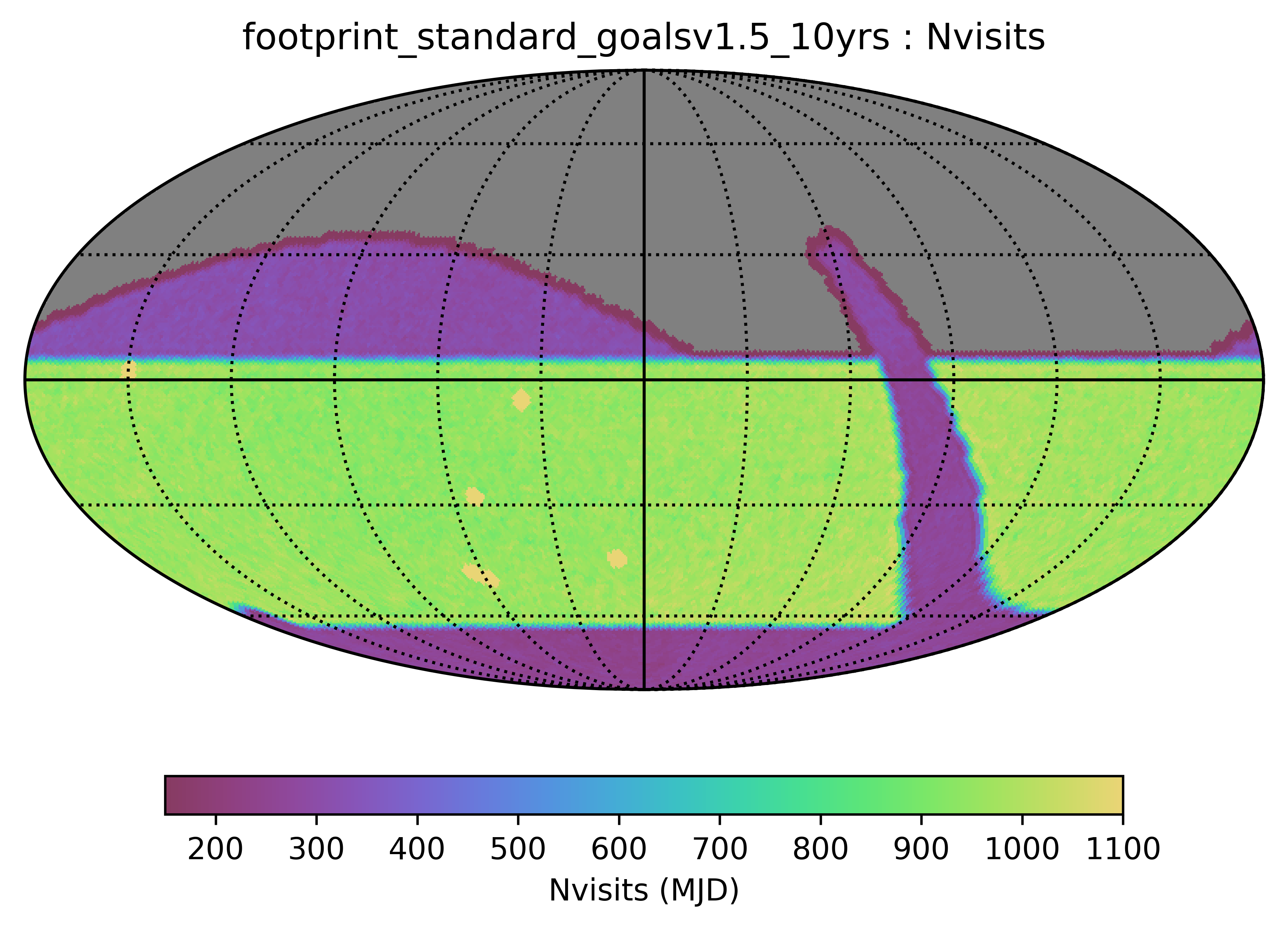
footprint_standard_goals is the same as baseline_v1.5, basically. This is the old standard survey footprint. The footprint_bluer_footprint survey uses this same map, however it has a bluer filter distribution (more u/g, less z/y).
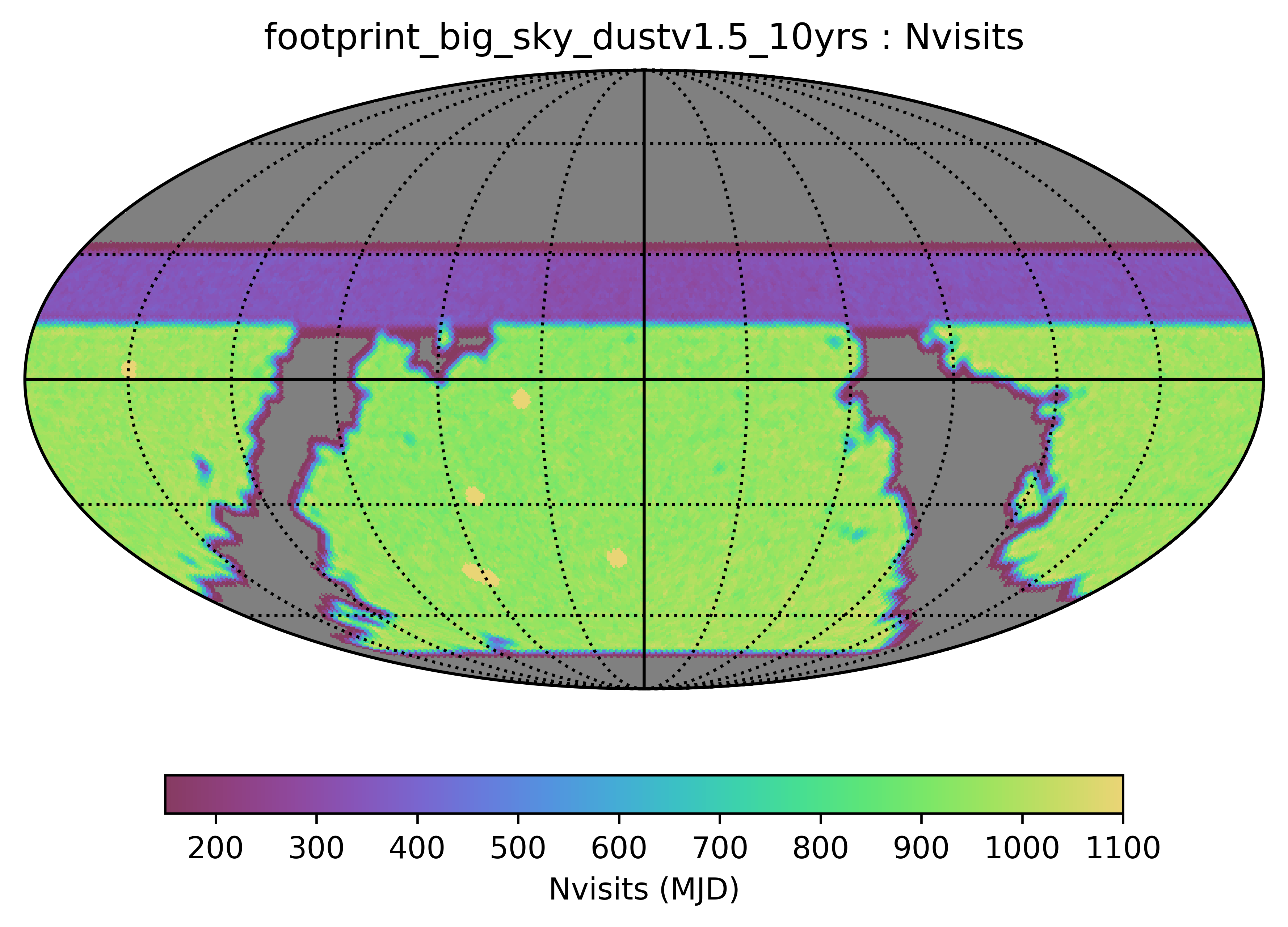
footprint_big_sky_dust uses an extended N/S region for the WFD (going about 10 degrees further north and south), with the galactic plane boundaries delinated by dust extinction. There is extended coverage with fewer visits to the north, but no SCP or galactic plane coverage.
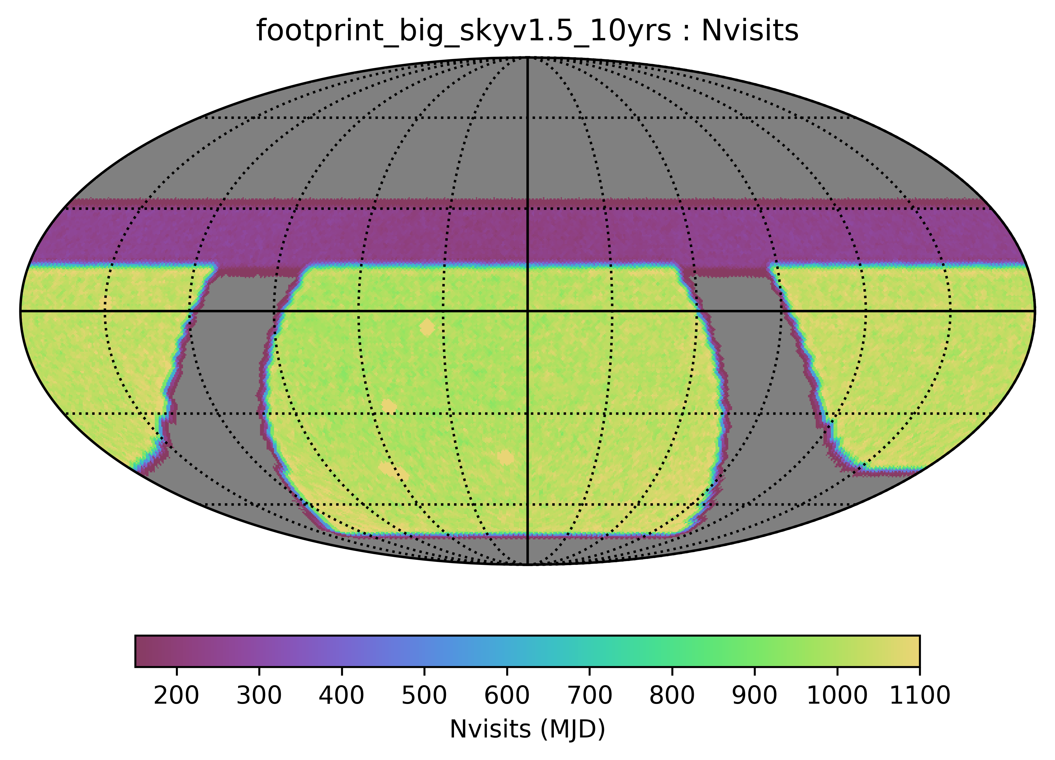
footprint_bigsky uses a similar extended N/S region for the WFD, with the galactic plane boundaries defined by a galactic latitude (=20deg) only. footprint_bigsky_nouiy is similar, but without u, i or y bands. Like in the footprint_bigsky_dust, there is extended coverage with fewer visits to the north, but no SCP or galactic plane coverage.
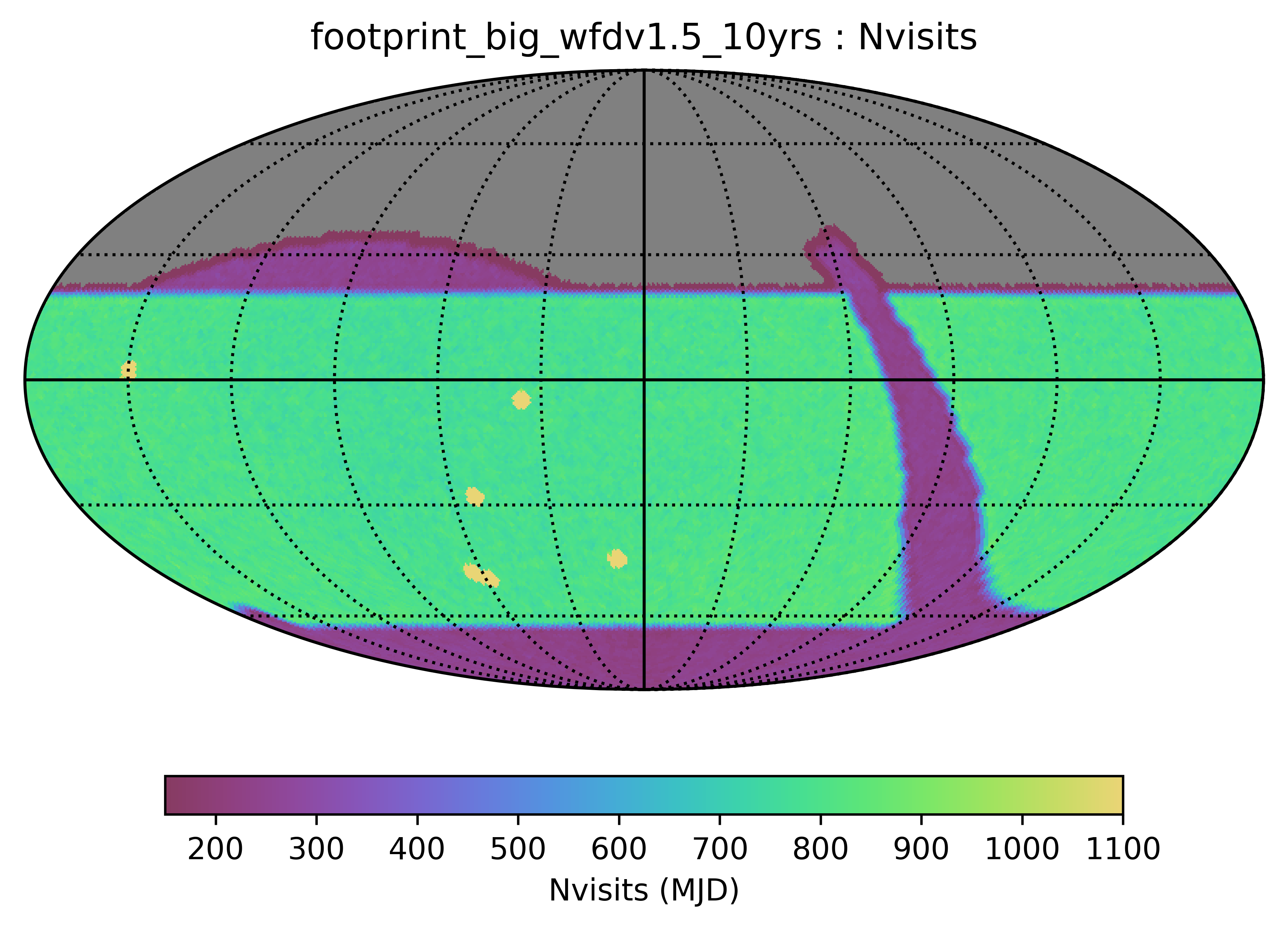
footprint_bigwfd is sort of a hybrid between the big sky and the standard survey; it has an extended WFD region, going further north than in the big sky but not as far south. This footprint includes SCP and GP coverage, with a small extension for the NES.
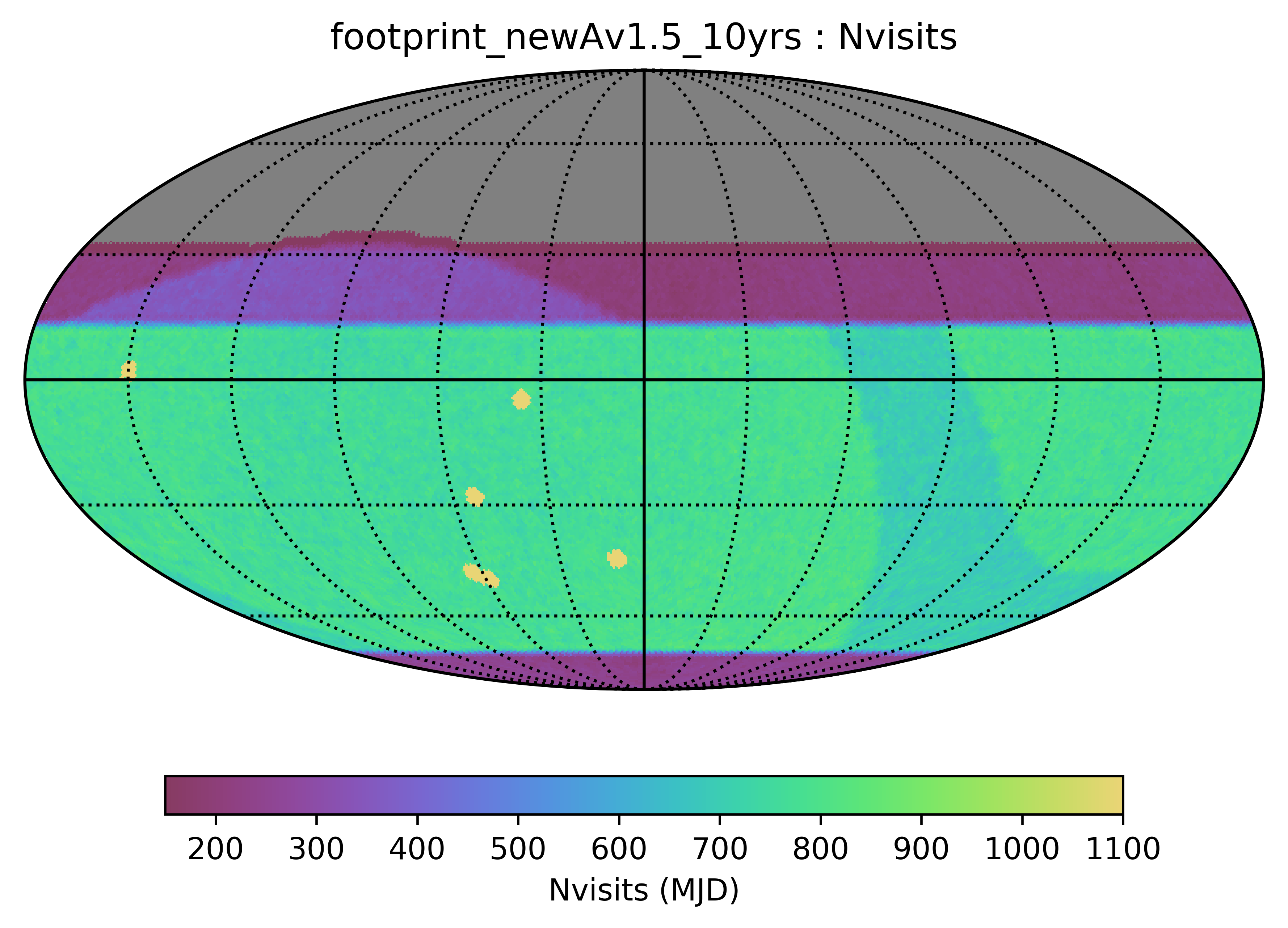
footprint_newA includes an extended N/S WFD (big sky style), with galactic plane region defined by galactic latitutde (l=20). The bulge direction is covered to slightly fewer visits than the full WFD; the anti-center is covered to normal WFD depths. The SCP and NES (and extended northern coverage) is included, to a more limited depth. The WFD region only achieves about 771 visits per pointing.
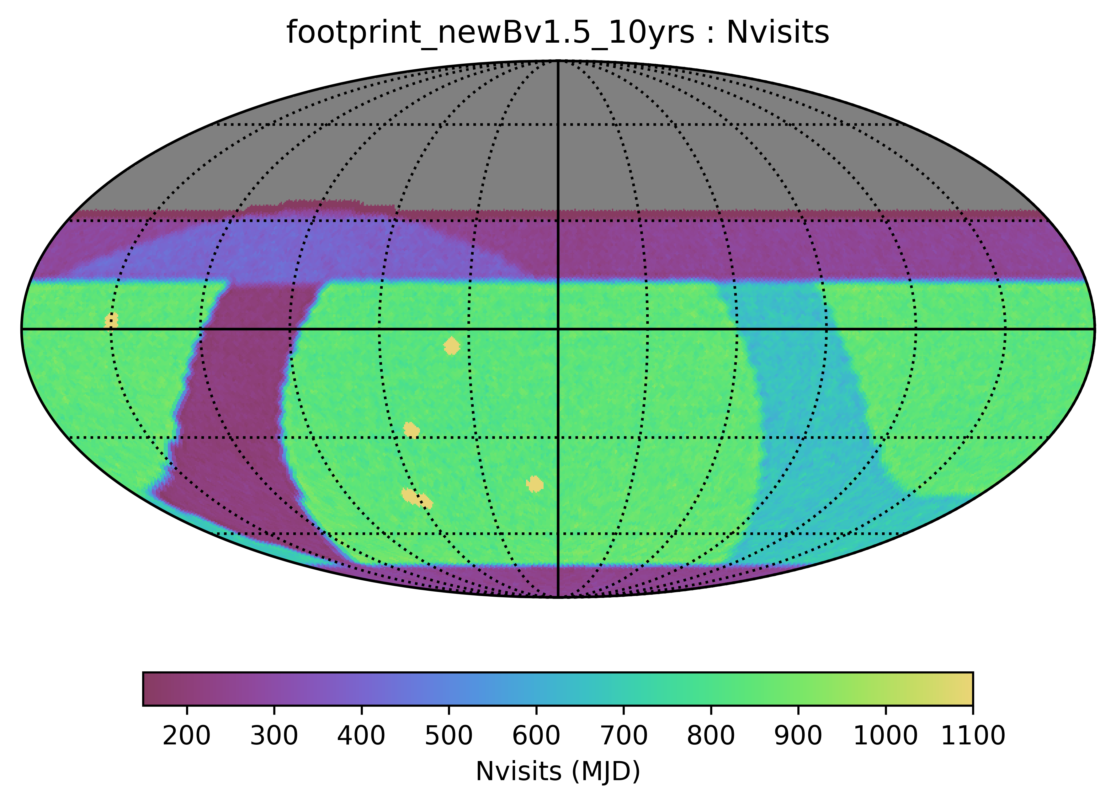
footprint_newB is similar to footprint_newA, but the galactic anti-center is covered to much fewer visits in an attempt to redistribute these into WFD and add to NES. The WFD region here achieves a median of 842 visits per pointing.
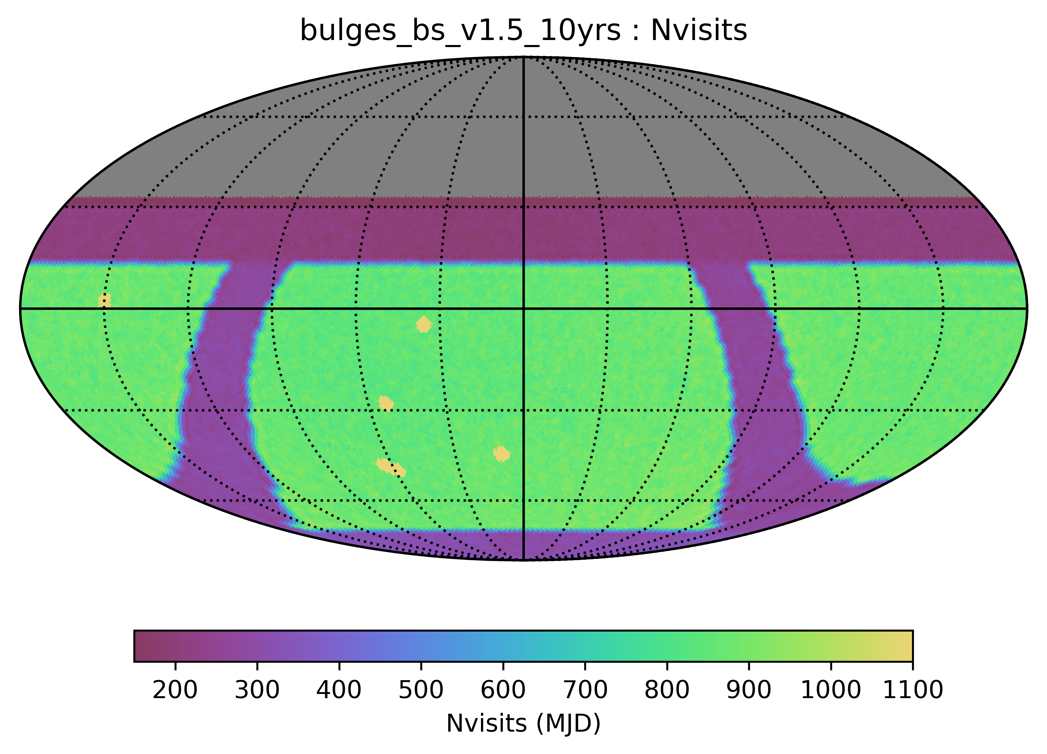
bulges_bs and bulges_cadence_bs use the same footprint map, although with different timing for the galactic plane coverage. Note that the WFD is extended N/S beyond the ‘standard’ footprint, so this is like the ‘big sky’ footprint, but with bulge, northern, and SCP coverage.
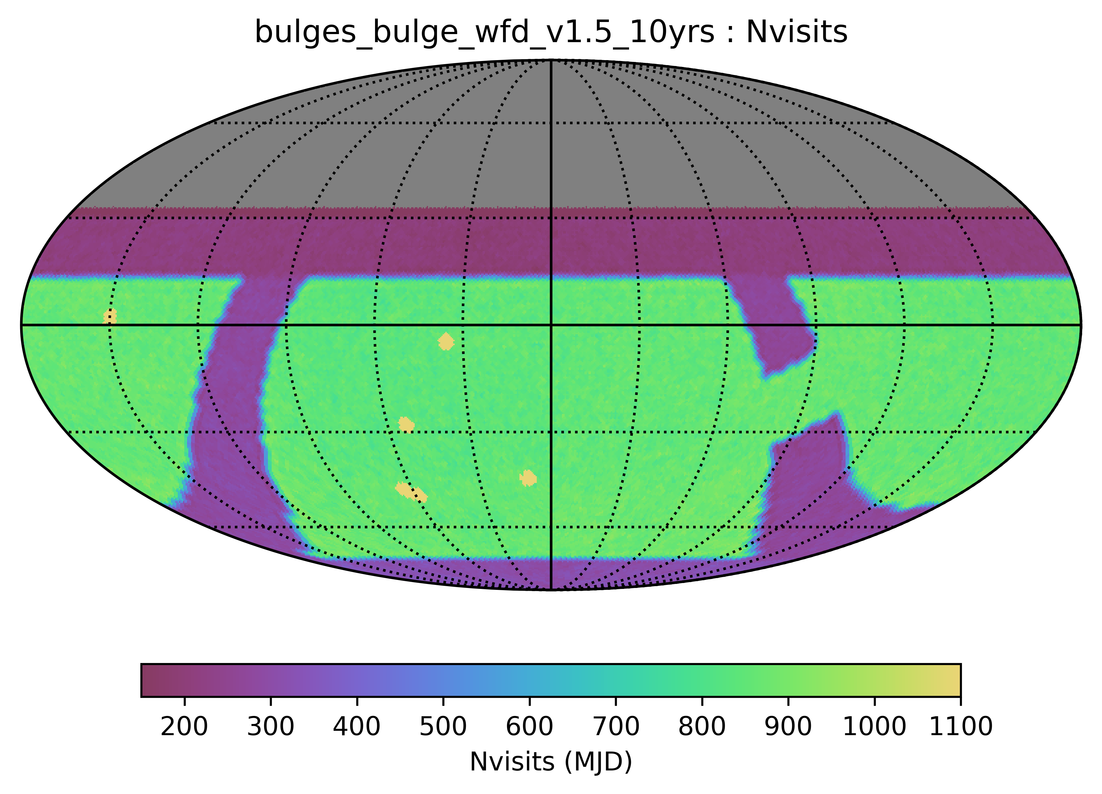
bulges_bulge_wfd and bulges_cadence_bulge_wfd, and bulges_i_heavy and bulges_i_heavy_cadence all use this survey footprint map, although with different timings and filter distributions. Note that it is similar to the big sky basis, but with galactic plane and SCP coverage, and these variations also have a band of WFD-level coverage through the galactic bulge.
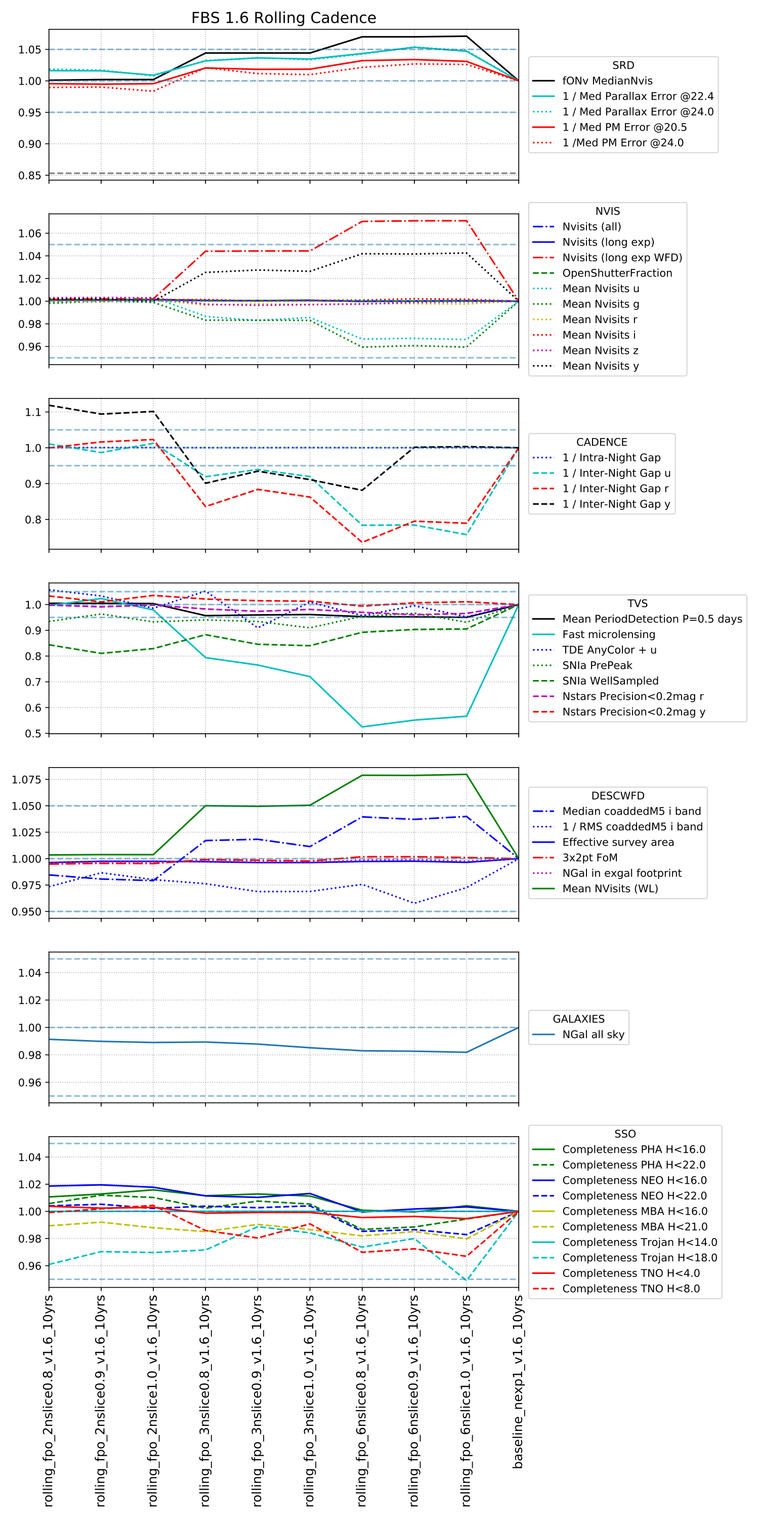
Rolling cadence – we look like we may need more metrics here. The 2 and 3 band versions don’t show huge differences compared to the baseline (no rolling). The 6 band shows some negative effects, and I would be concerned about vulnerability to bad weather (bad weather in one year would knock out one of the bands pretty significantly). There seems to be something we may not understand fully with the way the rolling cadence is implemented; it’s not clear to me why the fONv would increase with more rolling dec bands.
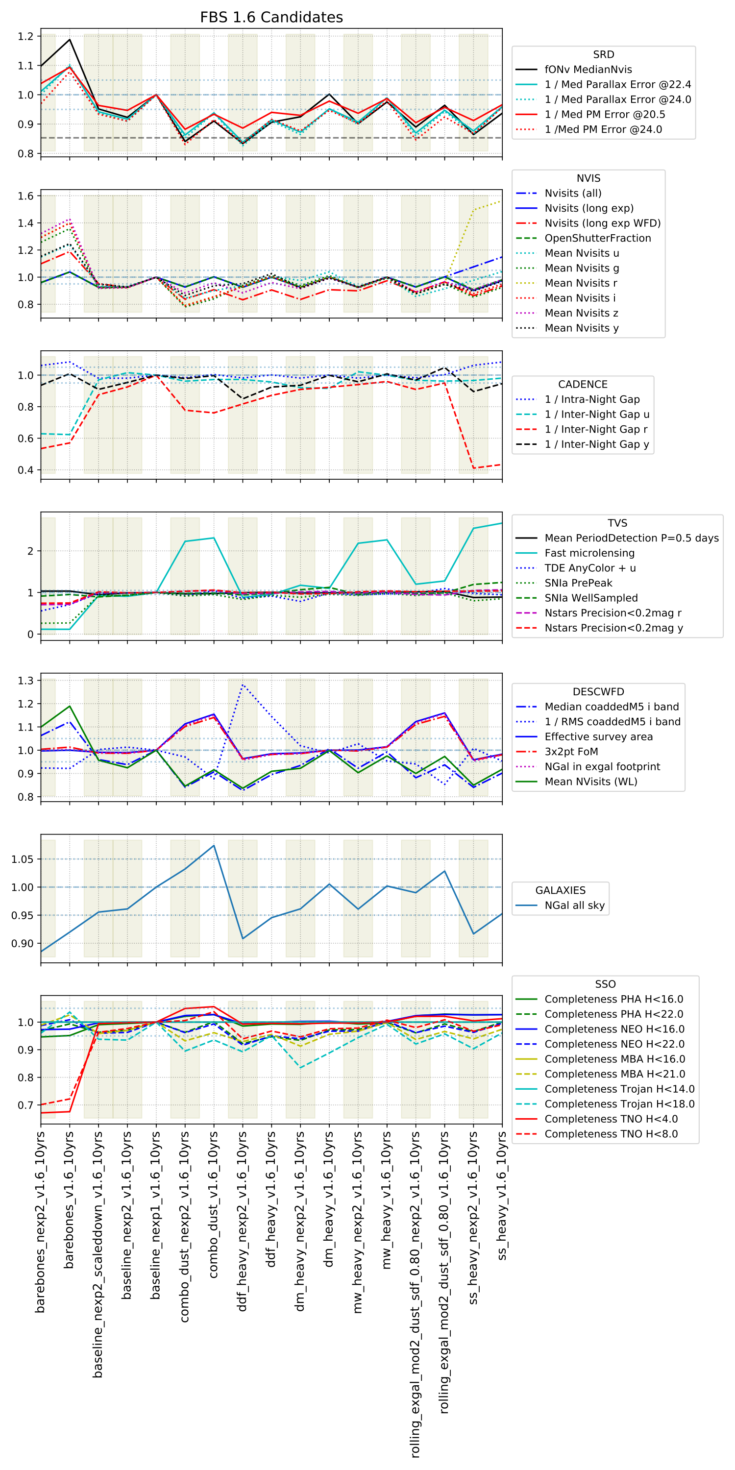
And the FBS 1.6 candidate runs … more about these in a different post, but to keep the metrics plot theme going.
We ran each of these simulations with 2x15s visits and with 1x30s visits; the shaded columns indicate the 2x15s runs and their corresponding 1x30s run follows in the next (right) unshaded column.