Visualizing OpSim output

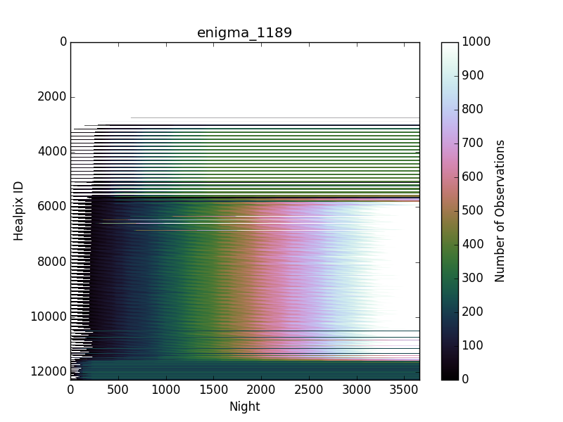
I started playing with a new way to visualize OpSim runs. Here’s a plot showing how many times a spot in the sky has been observed as a function of time. Normally, we just make Aitoff plots of various values at the end of the survey, but that doesn’t help if one wants to see the time-evolution. Basically, I’ve sacrificed displaying one of the spatial dimensions in favor of time here.

Some of the interesting things you can see:

  1. Large blue region at the top = outside the survey.
  2. region around healpix ID 4000 = North Ecliptic Spur. You can see it bumps up seasonally, and stops getting more visits after ~year 3.
  3. The big rainbow is the wide-fast-deep main survey.
  4. You can pick out a few of the deep drilling fields
  5. at the bottom, the South Pole gets observed less and completes early.

My hope is that plots like this might be a better way of doing quick visual Q&A on OpSim runs, rather than wade through lots of sky maps. And of course other things can be computed and presented like this as well (seeing, coadded depth, etc).

Comments welcome.

Can you upload a screen shot? I was trying to make visualizations that look somewhat like this

fig_firstSeason_0.pdf (19.1 KB)

My image should be embedded above now.

It is hard to decide how to include filter information as well…

This is sweet. It does nicely fold the time dimension down, though at the expense of some spatial context (though I guess folks will eventually get used to interpreting where there favourite Healpix tiles are).

One thought: how about showing an Aitoff map coloured by total visit integration beside the timelines axes you show. Then make some lines that go from key features along the right side of the timeline axes to locations on the Aitoff map?

I know this is controversial, but maybe let go of the jet colormap? palettable has lots of sweet colour maps you can use in matplotlib, including a totally flexible cubehelix map.

And maybe set the pixels with zero integration to np.nan so that you can get matplotlib to colour them as white so it’s easier to distinguish tiles that are completely missed from those that are only lightly integrated.

True, You have used the dimension I used for filters to show spatial variations, which is important for so many things.

  1. Is there high resolution information you wanted to capture by using healpixels rather than pointing fields?

  2. Don’t the cosmology DDF have many more visits than 1000 ? Are you treating 1000 as a ceiling (because otherwise color gets messed up)?

I was going to do it by field ID, but then I forgot that was my plan and subclassed the wrong slicer and just went with it. I’ll need to do a field ID version because that can easily be manipulated to check what fraction of observations are done in pairs, triples, quads, etc. The healpix version is going to be handy if we want to plot derived quantities as a function of time–e.g., as a function of time, how much area has reached a depth of X, or, what fraction of the sky has a good template image as a function of time.

yes, I set 1000 as a max to keep the color scale reasonable. I could try log scaling it I guess.

yeah, I’m so used to looking at raw IFU data that I don’t mind the spatial dimension jumble that much.

We’ve switched most of the MAF plots over to cubehelix. I still think jet looks better though.

And, it looks like matplotlib knows how to deal with masked numpy arrays, so I can just set my mask to True and don’t actually need nan’s.

I’m not sure having white be both maximum and minimum is that good an idea…

My personal favourite artisinally crafted cubehelix is perceptual_rainbow in palettable (full disclosure, I put it there so I’m biased).

And that’s the great thing about perceptual_rainbow! White is left for special uses. :boom:

1 Like

Ok that would be very useful. It is common in the cosmology DDF for there to be ~ 50 visits per night, with ~20 in each band . It would be nice to figure out if those were due to triples /quads or just OpSim deciding to do things that way. Maybe slightly unrelated, but it would be great to have a number of nights in independent filters metric in MAF.

That is better looking than most of the cubehelix things I’ve seen. Can I generate it with just matplotlib? We’re always trying to keep dependencies down.

This is a stripped-down version of what palettable is doing to make the perceptual rainbow colormap:

from matplotlib.colors import LinearSegmentedColormap
colors = [[135, 59, 97],
          [143, 64, 127],
          [143, 72, 157],
          [135, 85, 185],
          [121, 102, 207],
          [103, 123, 220],
          [84, 146, 223],
          [69, 170, 215],
          [59, 192, 197],
          [60, 210, 172],
          [71, 223, 145],
          [93, 229, 120],
          [124, 231, 103],
          [161, 227, 95],
          [198, 220, 100],
          [233, 213, 117]])
mpl_colors = []
for color in colors:
    mpl_colors.append(tuple([x / 255. for x in color]))
cmap = LinearSegmentedColormap.from_list('perceptual_rainbow', mpl_colors)

Drop that in a colormap factory function and you’re good to go!

Not bad.

I think I have to fiddle with the aspect ratio (or the dpi) a bit to make the lines a little thicker in the y-direction. I can see the deep drilling fields in the pdf, but not the png thumbnail.

1 Like

Would you mind sharing the code you used to make these plots?

Here’s a notebook where I tried to exercise all the vector metric functionality:

Hi, I want to suggest this is remade with a different color map: the rainbow color map is deceptive (not perceptually homogeneous) https://en.rockcontent.com/blog/rainbow-color-scales/

Hah ignore this! i am hella late to the party I see

Heh :slight_smile: 
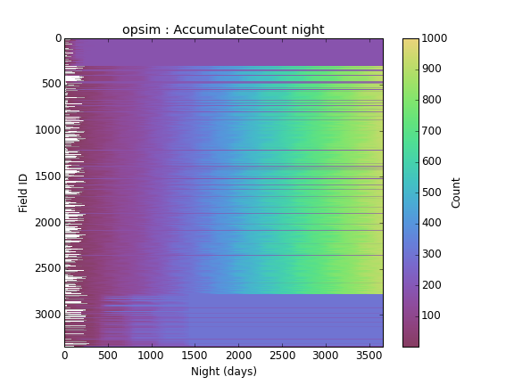
We have indeed swapped over to perceptual_rainbow.

1 Like