Light curves of stars and photometric calibration

[Paula (Paula Cáceres Burgos)]

Hi everyone

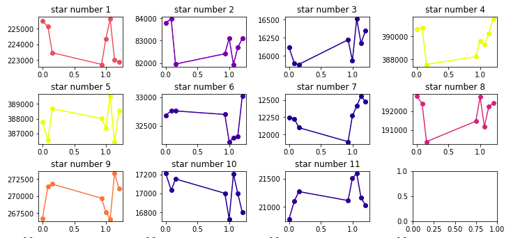
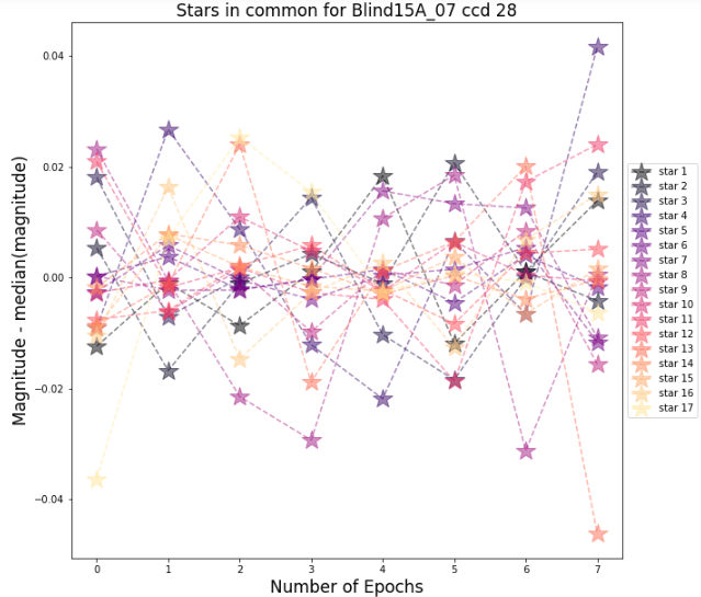
I’m currently analyzing the light curves I obtained by performing Image Differencing on DECam images. Right now, I want to ensure that non-variable stars show a flat light curve for all epochs, but for now, that doesn’t seem to be the case.

The stars I choose to plot come from a crossmatch between the src and the diasrc catalog of a given exposure, I select the ones that have 'src_calib_photometry_used' == True and 'ip_diffim_forced_PsfFlux_instFlux' is null. Because each image/observation uses a slightly different set of stars for the calibration, I only focus on the stars that are used for all epochs (and satisfy the constraints mentioned).

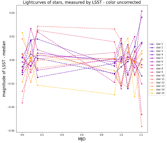
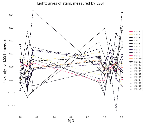
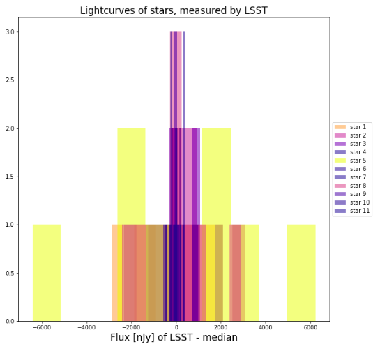
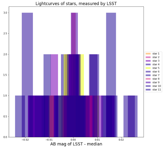
Here I show some plots, of course all of these fluxes and magnitudes are calibrated by the corresponding Photocalib method of the science image.

Here are the magnitude of the stars subtracted by their median, for every epoch (base_PsfFlux_mag). This value of magnitudes are obtained by calibrating the src catalog using the .calibrateCatalog method from PhotoCalib

Here are the fluxes in nJy of the stars for every epoch, I calculated it by multiplying the src column of base_PsfFlux_mag with the Calibration Mean of the corresponding exposure:

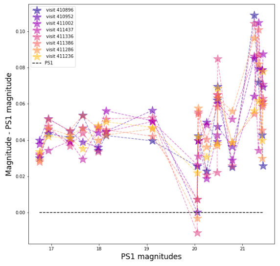
The variability of the magnitude of the stars are quite large, with a dispersion that gets to 0.04 magnitudes, I would like for these curves to be flatter, but I’m not sure how I could proceed or if its possivle. I wonder if the problem is that I should be looking at the set of stars used individually for each exposure? Instead of this smaller sample that’s not that flat, but I also think that eitherway they should look constant.

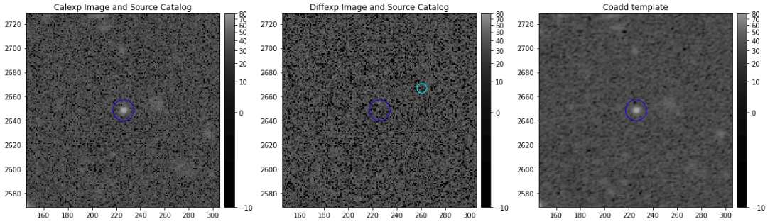
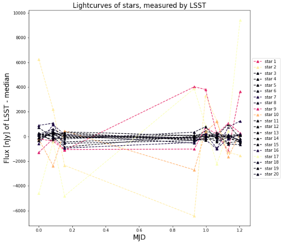
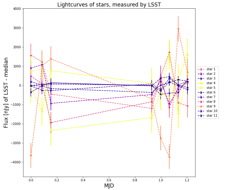
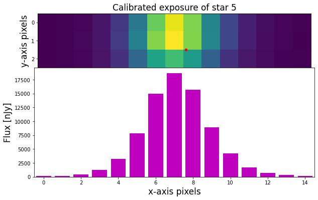
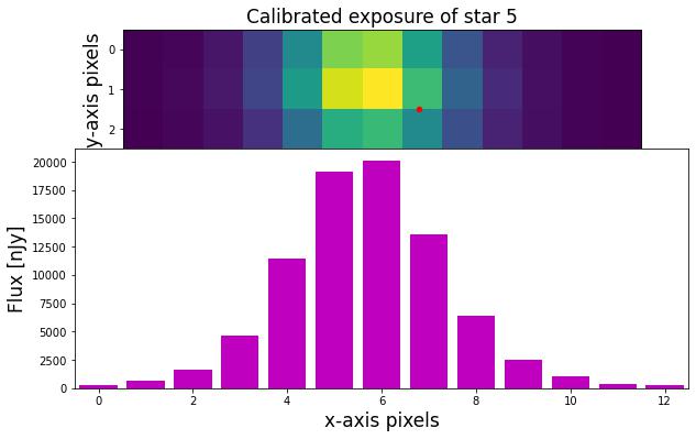
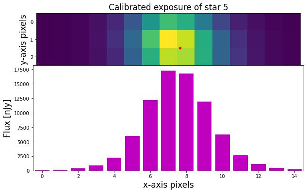
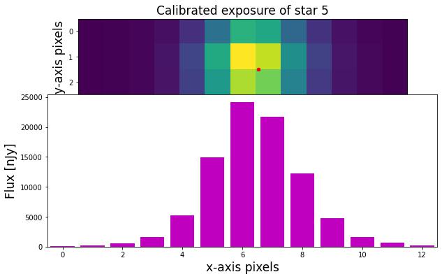
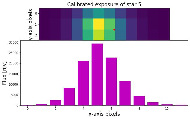
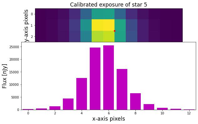
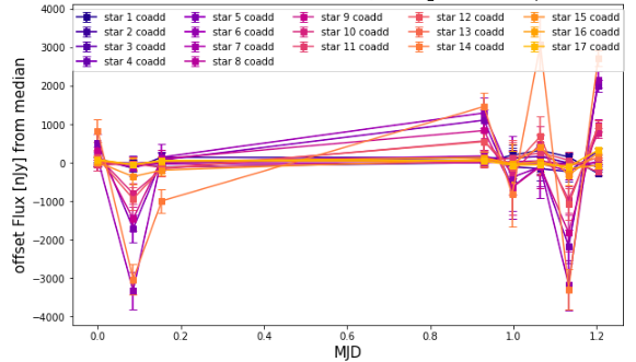
I also go ahead and measure the flux of the stars on the coadd exposure ('goodSeeingDiff_matchedExp') that is warped and psf-matched to the science image. Here are some plots:
The aperture I use is 2.5 times the PSF of the given exposure:

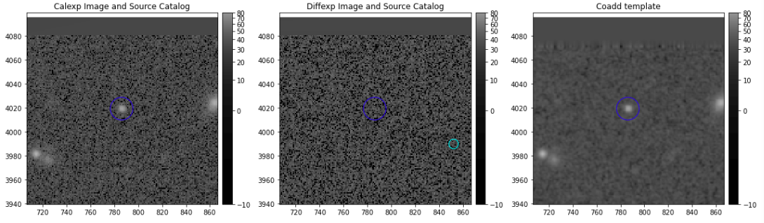
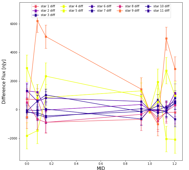
And here are the lightcurves of the stars on the difference image ('goodSeeingDiff_differenceExp') :

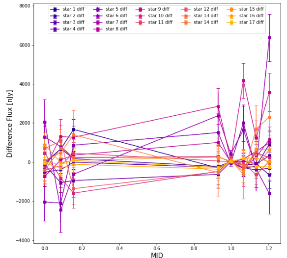
Also, lots of dispersion and tendencies.

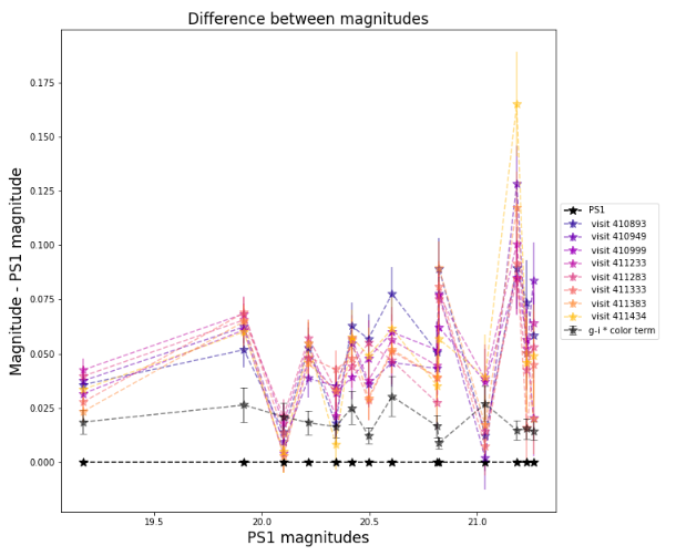
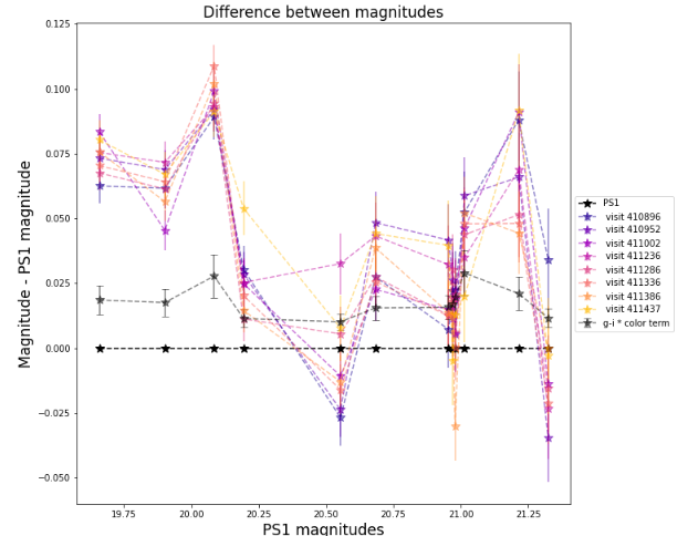
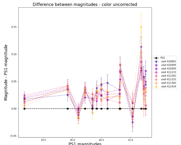
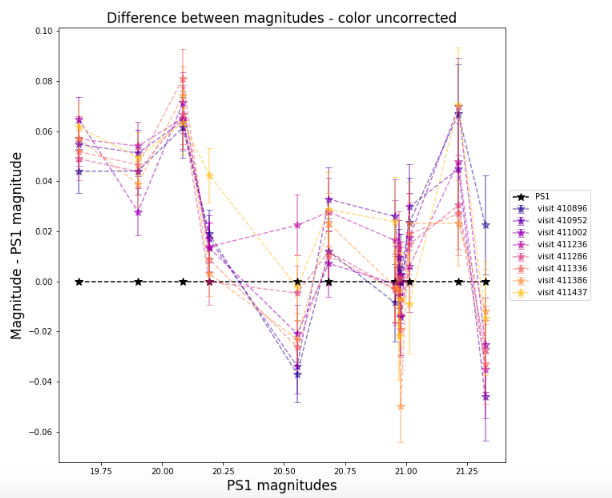
Another trial, and the last one is that I compare the magnitudes in GAIA with the magnitudes that are retrieved by the .CalibrateCatalog method on the src catalog:

The black star shows Gaia Magnitudes vs Gaia Magnitudes, and the other points are the stars found for each exposure. (the Gaia magnitudes are retrieved with Vizier query)

Happy to hear any comments about this!

Thanks

[parejkoj (John Parejko)]

What DECam filter is this?

Edit to add: What reference catalog did you calibrate the photometry against? Gaia is not a good choice for photometric calibration, as its filters are very different from most standard filters.

[Paula (Paula Cáceres Burgos)]

Is the g filter, and ok! I changed from Panstarss to Gaia because the newest versions of the software required the Gaia catalog, I guess this is just a default, and I can change it… I’ll redo the processing with panstarss as a test.

[Paula (Paula Cáceres Burgos)]

Ok, so I got it mixed up, sorry. I do use Panstarss for the photometric calibration, Gaia is used for the astrometry calibration (this is the default configuration). Here are the plots with the panstarss magnitudes:

It’s more consistent

If we look closely there is still great dispersion on the lightcurves of the stars, this plot below shows the magnitude of the star measured by LSST (found on the calibrated src table) subtracted by the corresponding panstarss magnitude vs. the panstarss magnitude.

[ebellm (Еrіс Веⅼⅼⅿ)]

@Paula

The stars I choose to plot come from a crossmatch between the src and the diasrc catalog of a given exposure

If you select only stars that also appear in the difference images, those will be variable by construction, so you shouldn’t expect flat lightcurves from them.

[Paula (Paula Cáceres Burgos)]

mmm this crossmatch is an ‘outer’ union between both tables, and I select the ones whose forced diffim psf inst flux (ip_diffim_forced_PsfFlux_instFlux) is null as a way to choose those correctly subtracted. Here are some stamps of the stars:

These stars are also the ones used for photometric calibration, so if it is the case that they are dia sources, at least in the coadd template, they should show a flat curve?

[Paula (Paula Cáceres Burgos)]

Hello

I checked that the structures found in the differences between the PS1 magnitudes and the ones measured by LSST here:

@Paula

can be somewhat explained by the color correction of the stars. Here are two plots that has the stars and the g-i color multiplied by the color term t

the color term that I used is t = 0.02, which is what I’ve found in the literature for DECam’s g band.
By subtracting the (g-i)*t (color * color_term) from the LSST magnitudes the curves get a bit more flat, but not that much…

maybe the color term should be larger? The stars that I use here are also generally faint, because those are the ones that are usually well subtracted. Many other bright stars show a dipole-type structure, which makes them a dia-source.

I wonder as well about the algorithm of finding the calibration scale (the factor that multiplied to the instrumental flux gives physical flux in nJy). I understand that It is found using a least squares, but are there any other treatments during the calibration, like a sigma clipping of saturated stars? or the ones that show very low signal?

Thanks for your time

[ljones (Lynne Jones)]

I was wondering about the star’s colors and their impact on the photometry here.
I am not super familiar with what is taken into account in the LSST photometric calibration tasks you’re using, but it’s interesting that the offsets got smaller when you added a color correction term (which I am thinking here means that the filter you’re using is different from the calibration catalog bandpasses, given that it’s just a correction for the color of the star itself), and so now I’m wondering if the position in the focal plane for the stars is also changing significantly between these observations?
I would expect a stellar color-dependent offset in the observed magnitudes of the stars resulting from changes in the atmospheric transmission, as well as location in the focal plane. I’m not sure what range of conditions is included here, how much variation in the stellar color is included, or how much the DECam bandpass changes over the focal plane though, so I don’t know how much variation to expect from those sources in this case.

[Paula (Paula Cáceres Burgos)]

@ljones

(which I am thinking here means that the filter you’re using is different from the calibration catalog bandpasses, given that it’s just a correction for the color of the star itself)

yes

@ljones

and so now I’m wondering if the position in the focal plane for the stars is also changing significantly between these observations?

I’m not sure how the position of the focal plane would affect the observed flux of the star… I’ll have to think more about it
The airmass does vary, here is a plot of that:

here is also the lightcurve of the stars measured by LSST and subtracted to its corresponding median:

I’m also not sure how much variation in the stellar color is included…

[parejkoj (John Parejko)]

@Paula

I’m not sure how the position of the focal plane would affect the observed flux of the star… I’ll have to think more about it

There is potentially significant variation across the focal plane, and we do not have a full focal plane transmission model for DECam (this would be generated by fgcmcal, but we are not yet able to run it on DECam). So all you have here are the single parameter per-detector fits. However, even those should have errors of only ~0.01 mags.

Are you running with a new enough Science Pipelines install to include the DECam colorterms (they were added in ~December 2021)? You should see a message like Applying color terms for filter=... in your logs. If you are not using the colorterms, that might explain the star-to-star variation when comparing with PS1.

[Paula (Paula Cáceres Burgos)]

@parejkoj

Are you running with a new enough Science Pipelines install to include the DECam colorterms (they were added in ~December 2021)? You should see a message like Applying color terms for filter=... in your logs. If you are not using the colorterms, that might explain the star-to-star variation when comparing with PS1.

I’m running it with the weekly version of lsstw_v22_29 (July 2022), and the color terms are added. I checked in the outputs from the pipeline:

lsst.calibrate.photoCal INFO: Applying color terms for filter='g DECam SDSS c0001 4720.0 1520.0', config.photoCatName=ps1_pv3_3pi_20170110 because config.applyColorTerms is True

[Paula (Paula Cáceres Burgos)]

I was thinking of this issue… could it be possible that the pipeline by default color corrects using a positive and fixed color term for all detectors? in other studies, it is found color terms by a given detector that can either be positive or negative.

[parejkoj (John Parejko)]

Yes, we only have a single color term correction for all of DECam to each of the refcats listed in this file: obs_decam/colorterms.py at main · lsst/obs_decam · GitHub

We do not have per-detector corrections, nor no way to handle or apply them. Even so, the differences you’re seeing for g band are much larger than the per-detector variation for DECam should be. What happens if you make similar plots for static sources in the src catalogs produced prior to difference imaging? Use exposure.photoCalib.calibrateCatalog(src) to get a catalog with all of the instFlux fields calibrated to nJy (using the matching exposure and src catalog, obviously).

[Paula (Paula Cáceres Burgos)]

Ok, Here is a similar plot of stars selected for photometric calibration by the pipeline before doing image differencing. I plot 20 random stars that are found in the 8 observations I’m working on.

the dispersion is roughly the same as the prior plot I showed. This plot is also now color-coded by their magnitude: for lowest magnitude (brighter stars) we have lighter colors, and for higher magnitude we have darker colors.

[parejkoj (John Parejko)]

Are you sure you have the units correct there? That looks like a dispersion of about 0.01 nJy, which is actually much better than I’d expect. I would expect a dispersion of a few nJy for single frame processing (575 nJy is ~24.5 AB magnitudes), not a fraction of a nJy.

It would be more helpful to plot these as a histogram of the flux dispersion, as measured across all sources with s/n > 50. You might be able to get something like this by running the MatchedVisitsQualityCore.yaml pipeline from the analysis_tools package.

[Paula (Paula Cáceres Burgos)]

yeah sorry!, your totally right, these are g-magnitudes on the y-axis. it is wrongly labeled :(, I can also add the plot in nJy

It’s a dispersion that gets to ±1000 nJy. The faintest stars here have around 21 g-mag.

@parejkoj

It would be more helpful to plot these as a histogram of the flux dispersion, as measured across all sources with s/n > 50. You might be able to get something like this by running the MatchedVisitsQualityCore.yaml pipeline from the analysis_tools package.

that would be nice! I’ll look into it

[Paula (Paula Cáceres Burgos)]

Ok, in the end I found easier to make a script that takes a horizontal rectangular slit of size 2*FWHM x 3pixels for a selection of stars used for photometric calibration by the pipeline. Then I take the median along the y-axis of the slit. These also have s/n > 50.

Here, the lightcurves of the stars on the science images before doing image-differencing:

The dispersion of ±1000nJy is still observed.

and the flux distribution of star 5

In this drive, I add the rest of the flux distributions of the stars.

I think is also useful to look at the lightcurves of the same stars in the difference image:

the variability observed in the calibrated exposures is somewhat retrieved but accentuated in magnitude, nevertheless.

[parejkoj (John Parejko)]

Why are you plotting cuts through the star image? When I said “histogram of the flux dispersion”, I meant “make a histogram of the dispersion in flux (flux - median) for all the stars in a patch brighter than s/n>50”. That way you can actually calculate the variation.

[Paula (Paula Cáceres Burgos)]

Oh, my bad. I misinterpreted the ‘across’. Thanks for the clarification

Here is the histogram. It is not the exact set of stars as the post before, sorry about that. Nonetheless, the color code criteria remain the same (brighter star → lighter color).

I also attach the same histogram, but in AB magnitude:

Looking at both plots, I see that the dispersion in nJy of the stars are just proportionate to the flux value of the sources. It’s imperative to consider the percentage of variation relative to the flux/magnitude value of the source itself. I will look into this

The range in magnitude for these stars goes from 17 to 21.