Dear survey enthusiasts,
We had previously thought the FBS 1.4 set of runs would be the last ‘big’ set with families/individual aspect survey strategy variations, but it turns out we were wrong – but for a positive reason. If you remember, most of our observations are taken as part of a “blob” Survey … this is the survey mode which activates for most of the footprint and for most of the time (except when weather conditions are unstable, such as during twilight). The “blob” survey chooses a portion of the sky that has the highest ‘reward’ function and then observes fields within this region over a given time span (about 20-40 minutes) and then repeats those fields in order to get a pair of visits in each night. In FBS 1.4 and prior, the choice of the fields within that ‘blob’ was based on the reward function (without consideration of location) and then the order was determined using a traveling salesman solution for efficient slewing. With FBS 1.5, we have experimented with adding an additional criteria – location of the field within the blob … more specifically, closeness to previously observed fields. This leads to observing contiguous/overlapping fields within each blob, which should increase the amount of sky available for rapid transient study, as well as hopefully improving SSO recovery. We found it also reduced the slew time significantly (well, the median dropped by 0.05s, but the mean fell by almost 1 second … which is significant when you have a lot of slews, and resulted in about 1% better open shutter fraction – a more efficient survey!). A 1% increase in efficiency is within our uncertainty on the weather … but we thought it was important enough that it was worth rerunning most of the FBS 1.4 runs with this new blob scheduling algorithm to let you compare.
Please note that we expect comparisons of metric results within families of FBS 1.4 runs to translate pretty directly to similar comparisons of families in FBS 1.5. Thus some families (in particular some related to new defaults we’ve adopted here in FBS 1.5) have been dropped in this FBS 1.5 run – but you could still look at the results in FBS 1.4 and the effects should be valid. However, if you would like us to recreate additional runs in FBS 1.5, please let us know. Comparison of runs between FBS 1.4 and FBS 1.5 (without normalizing by their respective baseline runs) is not a generally a good idea unless you’re looking for the specific difference induced by the change in blob scheduling.
As an example of the change in blob strategy, here is an alt-az plot of a night about halfway into the survey - you can see that the pointings are more contiguous in 1.5 than in 1.4:
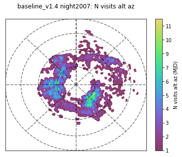
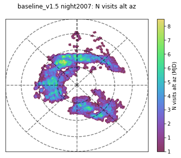
Alternately, here is movie comparison of the visits within an early night in the survey (night 50) in baseline_v1.4_10yrs (left) and baseline_v1.5_10yrs (right) to show the difference between FBS 1.4 and FBS 1.5 blob scheduling –
(there are some differences because the 1.4 baseline triggers a DD field early in the night, while the 1.5 baseline did not, but otherwise you can see how the ‘blobs’ in 1.4 are fields which are nearby, but not contiguous, while in 1.5 they are contiguous pointings).
Other changes in the overall default strategy have been implemented between FBS 1.4 and FBS 1.5:
- the u band filter is swapped out of the camera at 40% lunar illumination (about 6 or 7 days from new moon), instead of at 15%. This is in response to strong feedback from the transients community, who wanted more available time with u band in order to detect more transients. We do have a family of runs which experiment with this filter loading time however - please look into the filter_load and u_pairs families from the FBS 1.4 release if you think this will influence your metrics and let us know.
- Additional changes include that the u band visits are obtained in pairs, the default is to pair u band with a g or r band visit. This is in response to the need to characterize transients and variables, using more than just a single u band visit.
- Keeping the u band filter in the camera longer raised some concerns with the Deep Drilling field sequences, so now the DD fields are scheduled using a flexible-filter approach. Basically, we have a desired programmed sequence, that includes all of ugrizy in various combinations, and then whatever filter is not available in the camera when the DD is triggered is just skipped. This means that the gaps in coverage should have disappeared! We are experimenting with various DDF strategies based on requested strategies from the AGN and DESC groups and would welcome additional feedback and metrics. Variations on the DD strategy are available in DDFs.
- The default DDF strategy is updated to use visit sequences of ux8, gx20, rx10, ix20, zx26, and yx20 with whatever filters are mounted (so sequences will not include u or z depending on the moon phase). The DDFs comprise ~5% of the total visits.
- We removed the D290 DD field (which was our ‘placeholder’ DD field) and replaced it with the Euclid Deep Field South pointing – which translates to two Rubin Obs fields, so there are essentially two ‘new’ DD pointings which are treated as one. Our default is to take visits of this DDF in alternate years.
- Fixed a bug in the five sigma depth (m5) calculation when visits have 2 snaps – this means that baseline_2snaps_v1.5_10yrs is not 100% comparable to baseline_2snaps_v1.4_10yrs, but every other run should be fine.
Downloads
The FBS 1.5 simulations are available to download at either:
https://lsst-web.ncsa.illinois.edu/sim-data/sims_featureScheduler_runs1.5/
or
https://epyc.astro.washington.edu/~lynnej/opsim_downloads/fbs_1.5/ (these versions have an approximate labelling system for visits … see WFD metrics with the FBS output for more information on what this labelling could or could not help with). The links in the descriptions below go to this location for brevity, but the NCSA link is completely valid as well).
The directories contain ‘families’ of runs which aim to investigate a particular feature of interest in the survey strategy. The notes in each directory contain some information on the variation in question, and you can find in-depth information (via the actual python scheduler configuration scripts) for each run in https://github.com/lsst-sims/sims_featureScheduler_runs1.5
You can reach MAF metric analysis for these runs at:
http://astro-lsst-01.astro.washington.edu:8081/
There are several MAF output links for each run, including Metadata+ (a general collection of mostly metadata-related metrics, such as airmass, visit depth, etc. but also some SRD metrics), Glance (a very brief top-level set of metrics to check overall quality of the simulation), SSO (a collection of solar system object oriented metrics, which welcomes further expansion and input from the community) and ScienceRadar (a high level, science-oriented collection of metrics which also needs expansion and input from the community).
Family Summaries
A high level description of the families of simulations investigated in FBS 1.5.
-
baseline The baseline same-old ‘standard survey strategy’ run, which can be used as a general comparison point. Except for changes in the defaults, this stays the same from release to release and can be used to evaluate the effect of those default changes. There is a baseline using 1x30s visits (baseline_v1.5_10yrs) and one using 2x15s visits (baseline_2snaps_v1.5_10yrs). The project official baseline will remain 2x15s visits, so this is a good run to evaluate; however we have used the 1x30s visits as the default in the other families, so baseline_v1.5_10yrs is the one to use to compare survey strategy variation effects against ‘standard’ strategy. (for the final set of SCOC runs, we will use both 1x30s and 2x15s simulations for each of the potential candidate runs).
-
filter_dist This family varies the filter distribution across the standard WFD footprint – ie, taking more u band and less z or other variations. Our baseline filter distribution is nominally set to optimize photo-z measurements, but it would be nice to quantify how well photo-z and other transients perform with different filter distributions.
-
footprints This family varies the footprint of the survey - extending footprint for the WFD into the N/S, varying the coverage of the bulge, and adding Magellanic Clouds. These are sort of broad-stroke variations in footprint coverage, and it would be good to know if there are strong variations in your metrics with these - especially if they show that something might be particularly good or bad. The extended_dust footprint here is aligned with the request from DESC. The other footprints set up coverage in the north or south according to various white papers. These are generally a good set to investigate for everyone.
-
wfd_depth This family varies the emphasis on the WFD, using a standard survey strategy. The amount of time spent on the WFD scales up and down … while the time spent on other areas changes in response. This family is good for everyone to investigate, particularly if your metric primarily depends on WFD. It can be useful to see how your metric scales with the overall number of WFD visits or time. A similar set in FBS 1.4 may also be useful (but remember to scale by the relevant baseline) - in wfd_vary the time spent on WFD is held the same, but the area of the footprint is modified. In general, we think the footprints set above would serve the same purpose, but if you want more information that wfd_vary set may be interesting.
-
third_obs This family adds a third visit per night, in g, r or i, at the end of the night in the WFD (for some of the fields which had already gotten two visits earlier in the night). The amount of the night dedicated to this third visit varies across the family. If you have transient metrics, looking at the effect of adding this third visit would be very valuable.
-
rolling This family sets up a variety of options on rolling cadence - splitting the sky in 2, 3 or 6 different declination bands and alternating between these in different years, with either 10% or 20% ‘background’ level observations over the sky not included in the rolling footprint of the year. We have not really had a lot of feedback about these runs – if you are interested in transients and want a faster cadence (with the tradeoff of not observing part of the sky each year), have a look at these. So far, they do not seem very compelling.
-
alt_roll_dust This is yet another option/variation towards rolling cadence, but with an underlying ‘extended_dust’ footprint. The variations here are also a little different – one uses a simple two-band declination split, but the others with ‘alt’ in the name add an additional N/S variation (either on top of the 2-band rolling or without). The ‘alt’ runs are based on the strategy presented in the alt_scheduler, which chose a N or S region to focus on each night … what this means, in practice, is that there is a minimum 2-night cadence, and fields will not be revisited on adjacent nights. This adds some unusual features to the cadence which may or may not be problematic for people, depending on their science. We are particularly curious if this ‘alt’ strategy is good or bad for transient metrics.
-
DDFs This contains implementations of both the AGN and the DESC requested DD strategy. daily_ddf is another DDF strategy, attempting to take daily DDF visits. In these DDF sequences, we are now trying more aggressively to avoid the moon, although this may potentially cause more gaps in the sequences. We are still actively trying to develop the DDF strategy – if you are interested in the five standard DDF fields, investigate these families and let us know how this is working or not working.
-
goodseeing This family of simulations adds a reward based on acquiring ‘good seeing’ (seeingFwhmGeom ~< 0.7") images at each point on the sky, but varies in which filters this ‘good seeing’ visit is desired – one run just looks for a good seeing visit in i band while another looks for it in griz, etc. In general, I don’t think this family should have a major impact on most metrics, except metrics which require good seeing images (so maybe primarily metrics related to astrometry, lensing and weak lensing??). This family is good for everyone to check and for those who have metrics which should incorporate seeing, this family would be important to investigate.
-
u60 This run swaps 60 second u band visits for our standard 30 second visits. If you care about u band, you should definitely check this run.
-
var_expt This run changes the default exposure time per visit (becomes variable for every visit, between 20-100 seconds) to attempt to hold the single image visit depth roughly constant. This is worth checking for everyone, although it is not clear if DM will support this mode of operations.
-
spiders This run changes the distribution of the telescope rotation angle with respect to the camera. The concern is that DM may find it much easier and better to do image subtraction when the diffraction spikes from stars are aligned with the columns and rows of the camera - this constraints the telRot (telescope rotation angle) so that the telescope spiders align with the camera rows. The angle of the camera with respect to the sky will still vary, although in a more constrained way than in the standard baseline. People who worry about this should investigate this run and evaluate what they estimate the impact will be on science. I realize this is hard because the full effect on shear measurements, the most likely problem, from these angular distributions is not fully understood. It’s also worthwhile to note that this does not severely impact the overall number of visits, so it is also likely something we can wait to optimize until we have more information.
-
bulge This family of runs brings a variety of survey strategies to bear on the galactic bulge region. The names of the simulations are somewhat opaque, but include variations on cadence implementations in the bulge and also variations in filter distribution and overall number of visits. Everyone should check out this family, but if you are interested in science related to the galactic bulge, you need to look in depth at this family.
-
dcr This family adds additional high airmass observations each year to each point in the WFD, in various filters. This would allow DCR to be measured and corrected for in difference imaging, and potentially allow the measurement of astrometric shift caused by DCR for objects with sharp breaks in their SEDs (e.g., AGN with large emission lines). These runs are worth evaluating for everyone, but especially for people who are concerned with high-airmass visits.
-
Short exposures This family adds short exposures - either 1 second (
*_1expt) or 5 seconds (_5expt) long - over the entire sky in all filters either twice or five times per year (2nsor5ns). The number of visits in the entire survey increases – but some will be too short to be useful for some science – and the amount of time used for the mini-survey varies in each of these examples, from 0.5% to 5%. These runs are worth checking for everyone (the time requirement may impact your science), and if your science will benefit from these short exposures you should contribute some metrics. -
twilight_neo These runs investigate the effect of adding a mini-survey to search for NEOs during twilight time. The amount of time dedicated to this mini-survey varies across the simulations (depending on whether the search is run every night, every other night, or at wider intervals). These runs are worth checking for everyone (the time requirement may impact your science, even though the survey is run during twilight - we are currently using twilight time for some WFD visits), and particularly for solar system science.
-
greedy_footprint This simulation prevents the greedy survey from running on the ecliptic, instead pushing those visits into the ‘blob’ survey. This means the ecliptic will only be observed in pairs of visits, instead of the unpaired visits that occur during the greedy survey (which typically runs during twilight). Worth checking for everyone, and particularly for solar system science.
Happy simulation investigating! Please reach out (either here on community.lsst.org in the ‘survey strategy’ area or via email) for questions or help.
If the large number of runs seems overwhelming to you, I would suggest starting with a family that looks like it should impact your science and looking to see if your metrics reflect the changes you expected. If so, great. If not, why not? And then also running your metrics on the other families (or looking at our results, if you’ve already contributed and we ran your metric) and looking for any outliers. If you see runs that do particularly well or particularly poorly, why was that? If they all seem the same … is your metric not sensitive as expected (why not?) or is it just that the variations in the survey strategy don’t really impact your science (this happens not infrequently, due to the large number of visits)? Talk about it on community.lsst.org!
(in case this is also helpful - FBS 1.4 announcement and links).