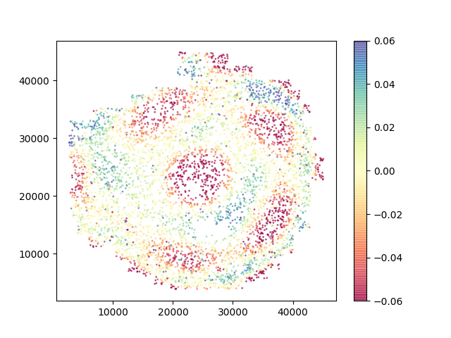
Dear all, we are using DM v19 to process some DECam data from raw, and compare the photometry (PSF mag) with DES. We use SkyMapper or PS1 (stars) as the photometric reference catalog, and Gaia as the astrometric reference catalog. The difference between the photometry of calexp_photocalib src from processCcd and DES looks random (Figure 1), but after running jointcal we found some pattern (Figure 2, 3 come from a dither group). The pattern is stronger in g and z-bands than r and i. This pattern changes with the number of input visits – if we use all archival data, we find some ring pattern (Figure 4), but it seems not from flat mastercals because it’s not centered and calexp doesn’t have this pattern. This pattern will propagate in coaddition steps and show up in the final coadd forced photometry catalog. (Figure 5)
We see similar patterns in other fields.
We wonder if anyone had seen similar pattern before. What should we do to avoid this, or is there any settings in jointcal we need to adjust (now we are mainly using the default config)? We appreciate any suggestions. Thank you.
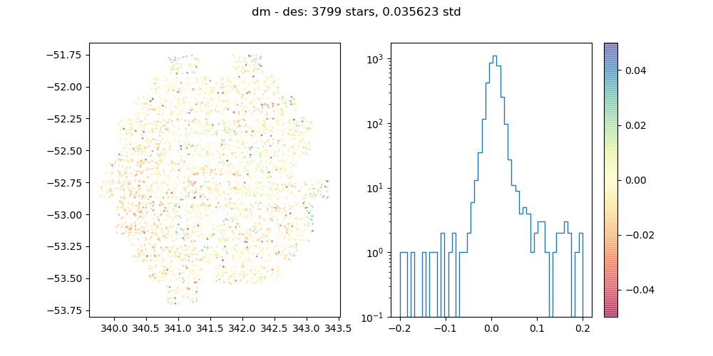
Figures: the Figure 1-4 are DES mag - DM mag (with shift), the Figure 5 is DM - DES.
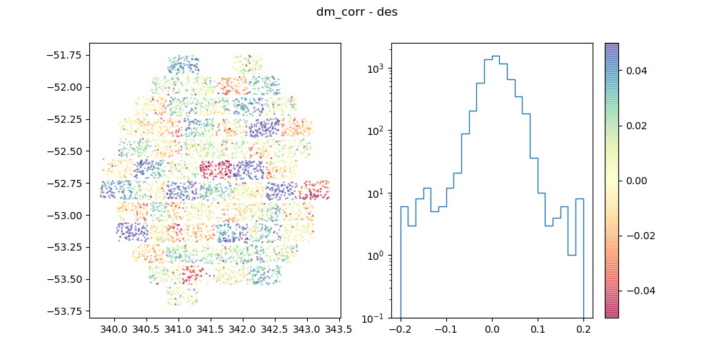
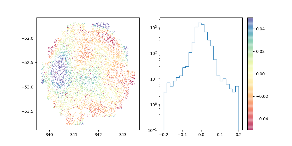
Figure 1: g-band visit 890702. The left panel shows the difference between calexp_photocalib src magnitudes and DES magnitudes (with a constant shift from color terms). The right panel is the histogram of the difference. We consider bright unsaturated stars between 16 and 20 magnitudes.
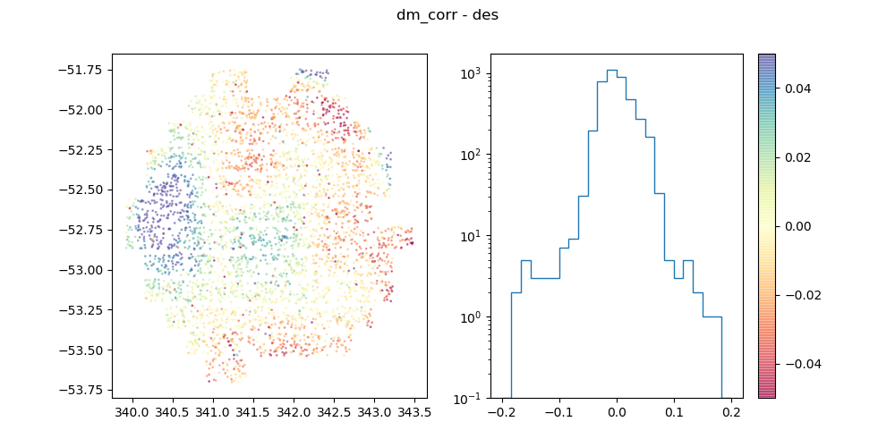
Figure 2: g-band visit 890702. We compare the jointcal_photocalib src magnitudes and DES. If we adjust wcs by jointcal_wcs, the result will be almost the same.
I am wondering if this is just noise in the calibration. How many calibration sources per chip are used, and what is the typical uncertainty (both catalog and instrumental) for those sources?
Thanks.
About 20-50 (photometric) calibration sources per chip in processCcd; 10-30 RefStars and 50-100 measuredStars per chip in jointcal.
The reference catalog is cleaned by flags and S/N>5.
The instrumental catalog is deeper and the S/N reaches tens or hundreds. The saturated stars are automatically filtered out.
Using SkyMapper and PS1 could both cause this pattern.
That SNR looks really low for photometric calibrations. For example, 20 stars with SNR~10 would provide a precision of 0.02 mags photometric calibration (at best). That’s not far from the offsets you are witnessing. I would check to see if many of your calibration stars are of a low SNR.
It may be that processCcd does a weighted mean which would help avoid low SNR stars. But it is worth inspecting none the less.
Single frame processing does not tie the detectors together at all, so the detector-to-detector variation will swamp any larger scale features.
We are mostly not using jointcal for photometric calibration in HSC processing now; it has been replaced by fgcmcal. Unfortunately, fgcmcal does not currently support DECam.
What do you mean by “If we adjust wcs by jointcal_wcs, the result will be almost the same.”? Do you mean you use the jointcal wcs output to correct the source positions before doing forced photometry on DES? I could see that having a small effect on the resulting comparison. Or this this just based on cross-matching of calibrated source catalogs, in which case correcting the DM coordinates with the jointcal WCS should have no effect on the comparison.
I wonder if you’re see the difference between the fluence and surface brightness here (I don’t know what DES reports): would it go away if you scale by the pixel area? Create an lsst.afw.math.PixelAreaBoundedField(bbox,wcs) and divide (or maybe multiply) each jointcal-calibrated source flux by the result of .evaluate(centroid).
Thanks. If we switch to DES as refcat, the result will be much smoother, but DES doesn’t cover some of the fields we are interested in. We also found that using DES as refcat in processCcd and then SkyMapper in jointcal could generate similar pattern, so it’s also possible the pattern came from refcat. If it’s only a noise, the pattern could be random, but we found it’s coherent.
to get magnitudes. Did it include the conversion between fluence and surface brightness? The scale by the pixel area could be monotonic radially, which is different from the pattern.
Can I ask the definition of bbox and centroid?
Could you point us to any document that gives more details about these commands?
Is there any parameter in jointcal’s config that’s worth adjusting? (e.g. the order of some polynomial)
Thanks.
Thanks for pointing this out. I’m not sure if PS2 catalog has been published. If so, could you point me to it? Also, the coverage of PS1 is DEC>-30 deg, but some of the regions we are interested in have DEC<-30 deg…
From your description, I don’t know if you were doing forced photometry or just cross matching DM and DES catalogs. If the latter, updating the coordinates should not have any effect on the photometry difference (you might gain a few more matches, but the photometry values will be unchanged). If the former, it might have a very small effect, but I don’t have a good way to quantify it.
Per the Community page I linked, jointcal’s photoCalib is always fluence. The pixel scale from the jointcal WCS fit is definitely not radially monotonic.
bbox is the bounding box of the exposure (e.g. exposure.getBBox()), and centroid is the x/y pixel center of the source being corrected.
The PixelAreaBoundedField docs may or may not be helpful to you. We don’t have any further docs on using them, as this particular situation hasn’t come up, and fgcmcal is more explicit in how it includes the pixel area effect.
You could try increasing the photometryVisitOrder config option, but I’d be somewhat surprised if that fixes it, given that the differences in your images are relatively slowly varying.
What surprises me the most about this is that the scale of the DM vs. DES photometry difference appears similar between the single frame and jointcal PhotoCalibs. I’d have expected the ccd-to-ccd differences from single frame to be much larger than any residual difference from jointcal. Have you computed a variance statistic? The scale bars on your plots are the same from plot to plot, which is good, but it’s a bit hard to get a feel for how much (if at all) the scale of the difference has moved. Overplotting the histograms, and/or plotting them in flux instead of magnitude space might help with that.
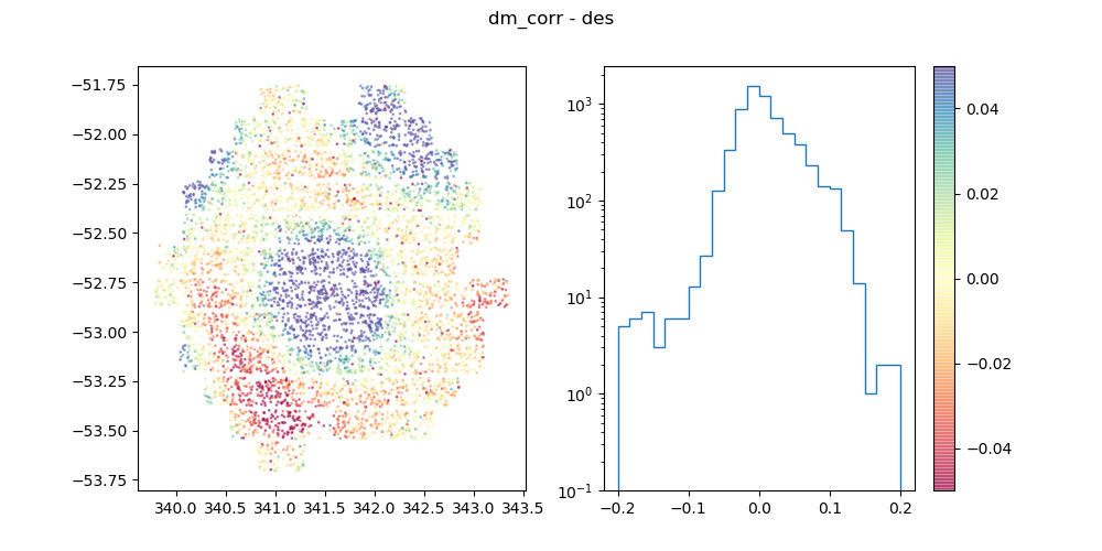
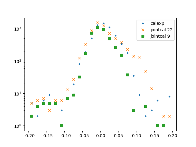
Figure 2 to 4 above show the difference between DM jointcal calibrated catalog (one visit; this is before co-addition) and DES catalog after spatially matching the coordinate of stars. Figure 2 and 3 run jointcal on 9 high-quality visits (a dither group; they are not DES exposures). Figure 4 run jointcal on 22 visits (including some short exposures with telescope pointing centers far from the dither group).
Figure 5 above gives the result of running jointcal on the 22 visits → coaddition → forcedphotometry.
If we only use those 9 visits (dither group) and then jointcal → coaddition → forcedphotometry, the result will look like this (similar to Figure 1 and 2). We think the pattern appears at jointcal and propagates into later steps.
For example, visit 890702 in Figure 1 has standard deviation 0.046 mag, in Figure 2 the standard deviation is 0.041 mag, in Figure 4 it’s 0.054. Here is the result of putting the histograms together.
The refcat depth could be one reason as Wesley pointed out, and the short exposures with distant pointing centers can be another one.
It looks the pattern moves with stars (Figure 2, 3), so we suspect the pattern might partially come from the refcat/celestial objects or blending, but we need more investigation.
We found in jointcal photometryVisitOrder config parameter (“Order of the per-visit polynomial transform for the constrained photometry model.”) at 2 gave the best performance (the default value is 7). This is true for both g-band and z-band. Here is an example: g-band visit 890702 jointcal-calibrated magnitudes compared with DES. In this jointcal run, we used all archival data.
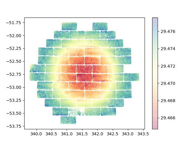
We used these commands to obtain the scale by the pixel area.
calexp = butler.get("calexp", **dataId0)
bbox = calexp.getBBox()
wcs = calexp.getWcs()
var = lsst.afw.math.PixelAreaBoundedField(bbox, wcs)
value = var.evaluate( src.getX(), src.getY() )
We used -2.5*log10 to convert the value into a magnitude (for comparison with the results above), and the range of the value is ~ 0.01. Here is the image (of the same visit).