Rubin Seeing Band Distribution

[pollack (Jennifer Pollack)]

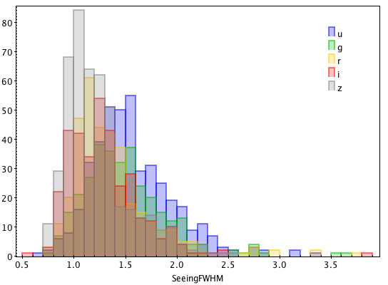
I am covering for someone (now on leave) who was preparing Rubin survey target files for image simulations of Euclid targets as observed by the Rubin Observatory LSST camera. I have attached a plot using the seeingFWHM column from survey files that were provided to us. There appears to be too many high values to be realistic for Rubin. I was hoping someone could have a look and let me know whether or not this looks correct?

[boutigny (Dominique Boutigny)]

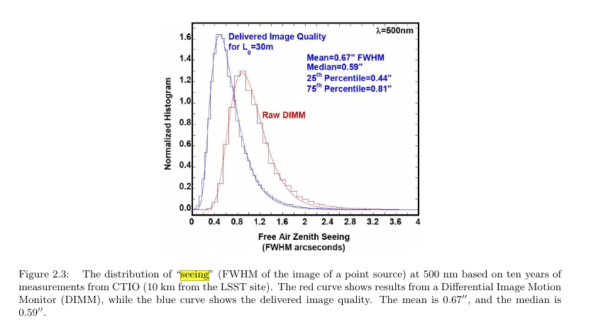
Here is a picture extracted from the LSST Science Book (page 29). It is for a wavelength of 500 nm but it looks to me that the seeing FWHM distribution that you are using is shifted toward too high values.

[pollack (Jennifer Pollack)]

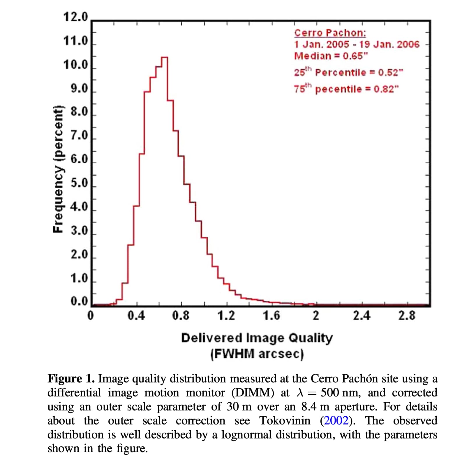
Yes, thanks. that’s what we thought. We also consulted a similar plot in this paper https://iopscience.iop.org/article/10.3847/1538-4357/ab042c/pdf). We found that rescaling the seeing down by a factor 1.7 or 1.8 (depending on band) gave us the seeing distributions in the survey files with the same median (and similar scatter) to that discussed in this 2019 publication.

[cheymans (Catherine Heymans)]

Hi Jennifer,
Would it be possible for me to download the raw data for these seeing distributions (modulo the rescaling correction factor that you found that you needed). I’m hoping to use them for a “back of the envelope” calculation for how the variable depth in DR2 might to fold through to the weak lensing analysis.
Many thanks in advance,
Catherine

[yoachim (Peter Yoachim)]

Here’s a handy plot I made a while back looking that the seeing distribution in different filters.
seeing_dist_all.pdf (25.7 KB)

Note that the cadence simulations have columns of seeingFwhmEff and seeingFwhmGeom. Documentation on the difference between them should be here: Scheduler Output Schema — rubin_sim Current documentation

[pollack (Jennifer Pollack)]

Hi Catherine,
The raw Rubin-like data is stored in the Euclid Archive System, and unfortunately it is currently only accessible to members of the Euclid Consortium (EC). If you are an EC member, I can get you the info for how to access them. Just let me know.

Best Regards,
Jennifer

[ljones (Lynne Jones)]

Hi Catherine - are you looking for Euclid data or are you looking for Rubin data?
If you are looking for Rubin simulated seeing distribution data, we can provide that. @yoachim gave you a link to a PDF plotting the ‘delivered’ seeing from the simulations, but you can also access a variety of other items.

It may be worth noting (and this may be relevant for Jennifer as well) that there are a couple of things we can provide:

• a simulated raw 500nm zenith ‘seeing’ distribution for the lifetime of the LSST (find this in the tar file at this link: https://lsst.ncsa.illinois.edu/sim-data/rubin_sim_data/site_models_may_2021.tgz – this contains a sqlite database file called ‘seeing.db’ which contains the equivalent of 500nm zenith ‘atmosphere only’ seeing measurements (the columns are time in seconds, DIMM seeing in ", take the time as starting at January 1 of any year)

sqlite> select * from Seeing limit 5;
seeingId|s_date|seeing
1|0|0.782576024532318
2|300|0.872810006141663
3|600|0.746892988681793
4|900|0.851306021213531
5|1200|0.720582008361816

We use this 500nm zenith seeing combined with a model of how the telescope optics and dome, as well as airmass and filter choice, combine to create a ‘delivered’ seeing for each image.
The model is implemented here: rubin_sim/seeingModel.py at main · lsst/rubin_sim · GitHub
This raw distribution is however, unlikely what you actually want to use, because you most likely want to fold in the actual survey strategy / location of visits, etc.

• More likely, what would be appropriate would be the delivered seeing measurements that are part of the opsim outputs. These opsim outputs contain a simulated pointing history for the LSST, from which you could pull out the seeing distribution at any point in the sky in any single (or multiple) filters. If you have a measurement you want to make using this information, MAF may be an excellent tool to add in (if you don’t know what MAF is, we can point you to some more documentation here if you want). As @yoachim described above, there are two columns in these outputs which are relevant – the seeingFwhmGeom and seeingFwhmEff. Depending on what you want to do with the seeing value, you may want to use one or the other or potentially both (seeingFwhmEff represents more closely the number of effective pixels in an image that contribute to SNR for a point source; seeingFwhmGeom represents more closely the physical size of a point source profile if you assume a simple double-gaussian PSF). You can download a sqlite file containing the current baseline survey simulation here - http://astro-lsst-01.astro.washington.edu:8080/fbs_db/baseline/baseline_v2.0_10yrs.db

sqlite> select observationStartMJD, filter, airmass, seeingFwhmEff, seeingFwhmGeom from observations limit 5;
observationStartMJD|filter|airmass|seeingFwhmEff|seeingFwhmGeom
60218.0018055556|y|1.17253420858044|0.748625780318801|0.667370391422055
60218.0022541388|y|1.20704594211365|0.761769790309123|0.678174767634099
60218.0027027933|y|1.24818961117279|0.777244761537956|0.6908951939842
60218.0031515168|y|1.29560474381897|1.95333303256225|1.65763975276617
60218.0036237433|y|1.37148119736193|2.02118790858406|1.7134164608561

[ljones (Lynne Jones)]

BTW, The rescaling factor that Jennifer mentioned may be part of the fact that the plot linked above seems to be the 500nm zenith measurements, not the actual ‘delivered’ image seeing values.
I’m not sure exactly which plot you were referencing from the 2019 “LSST Overview paper” but if it was this one -

then that is also only the 500nm zenith measurements, and again does not include the contributions from the telescope and dome, airmass of an observation or the filter choice (so I would expect the values to be both more narrowly distributed than the simulated delivered image seeing and also have a lower median value). Peter’s linked PDF above - seeing_dist_all.pdf would represent the distribution of delivered seeing, once you add in these additional factors.

[ljones (Lynne Jones)]

I’m sorry we missed your original message from 2021 … I’m not sure which simulation this came from, but it is possible that some images were acquired with pretty high seeing values. It might be worthwhile to recreate this plot with the data from a newer simulation.

[pollack (Jennifer Pollack)]

Thanks so much, Lynne. I have a question about MAF and it’s application for DESC DC2. Were rotational and translational dithering applied to the entire WFD area or just the DC2 300 sq. deg region? I am asking because we would like to add rotational dithering to the Euclid Rubin-like simulations. It would be great to know how to use the MAF to implement this feature.

[ljones (Lynne Jones)]

I’m not sure - I think it was likely the entire sky and then they subselected the visits of interest, but their process could have worked in reverse too.

You could use a MAF stacker to add rotational dithering. Then though, you’d still need to write out the updated visits into a new copy of the database, if you want to keep that information between runs.
An example rotational dither stacker is here: rubin_sim/ditherStackers.py at main · lsst/rubin_sim · GitHub
however, I’m noticing that that stacker only changes the rotTelPos, not rotSkyPos (which should change at the same time). There are some limits to the rotational positions that are allowed, and there is some time cost to rotating – which isn’t captured when using a stacker rather than actually adding it to the scheduler.

This may be obvious, but when we want to change the actual dithering plan, we update it in the scheduler not MAF. The tests with MAF were for cases where it was good enough to have something approximate, to guide further investigations going into the scheduler (and also from a time period where dithering wasn’t implemented in the scheduler at all).

[ljones (Lynne Jones)]

Just to link in the DC2 visit information (with DC2 dithers added):
https://lsst.ncsa.illinois.edu/sim-data/desc_dc2/minion_1016_desc_dithered_v4_trimmed.db

[pollack (Jennifer Pollack)]

Hi Lynne, Hi @yoachim,
Thanks. For the moment, we decided to go with the nominal settings for translation and camera rotation in the baseline_v2.0_10years run.

Yesterday, I sent Lynne a pm but in case she is busy or on holiday I decided to post here to see if Peter or someone else can answer. The Euclid Consortium simulation group is working on a paper describing the Euclid simulation framework and will present results from their Scientific Challenge 8, which took place last year. For this challenge, we simulated Rubin visits using the OpSim output: footprint_big_sky_dustv1.5_10yrs. Can you let us know how we should cite OpSim? Thanks a lot.

[ljones (Lynne Jones)]

Citing opsim is a question we have been talking about lately, as a more up-to-date reference would be good.
The citations needed can be found here: LSSTreferences/LSSTreferences.pdf at master · lsst-pst/LSSTreferences · GitHub in section 3 (and if you go up to GitHub - lsst-pst/LSSTreferences: A package containing all LSST BibTeX entries - Cite LSST you will find the bibtex entries conveniently located in LSSTbiblio.bib).

Much of the opsim framework and supporting modules were developed under the LSST simulations effort, so citing the effort using the LSST simulations overview paper (Connolly et al 2014) is appropriate. Then the feature based scheduler itself is cited as Naghib et al 2019, and it would probably be worthwhile to throw in the older opsim reference of Delgado and Reuter 2016. The opsim run you mention can be cited as Jones et al 2020.

That’s a lot, so one possible way to word it might be:
"The LSST scheduler (Naghib et al 2019) and associated simulated pointing histories (‘Opsim outputs’) (Delgado and Reuter 2016, Connolly et al 2014) provide many examples of survey strategy options. For this work, we used the output from the v1.5 simulation, `footprint_big_sky_dustv1.5_10yrs’ (Jones et al 2020). "