Source injection variance

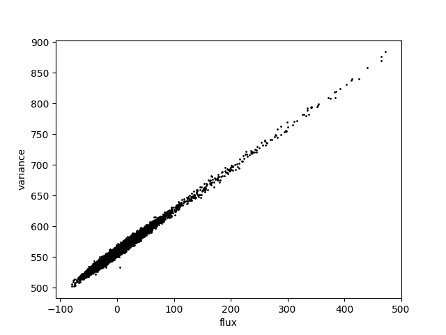
I am doing source injection on visit images in DP1 and I noticed a strange behaviour in the variance maps. Here I have a small cutout (128x128 pixels) before injection and I plot the variance vs the flux:
data_variance_rubin

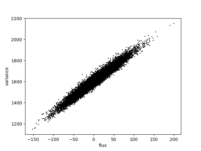
this looks like I expect, basically a linear relation with maybe some calibration/gain differences. However once I run the source injection pipeline task the sample plot looks like this:

data_variance_rubin

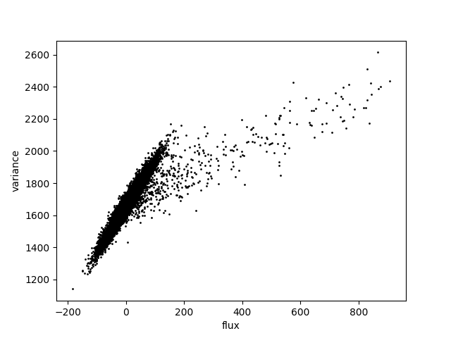
It’s not really following the trend anymore. Obviously I have injected a pretty bright object in the cutout, but still I would have expected it to follow the same trend.

In case it’s relevant:

  • This is a u-band image. I haven’t checked others but I can
  • I injected a point source, just using the default PSF model for the visit image, at the appropriate position etc.
  • The objectID where I’m doing the injecting is: 592914119179383718
  • I’m using the injection task from lsst.source.injection import VisitInjectConfig, VisitInjectTask
  • The original and injected images aren’t perfectly aligned, they will be offset by 2 arcsec since the inject one is centered on my injected point source. Still, my injected point source is by far the brightest in the cutout so the high flux values are definitely injected ones

Isn’t it just the quadrature addition of the two noise sources (the linear addition of their variance)? In that case, given the variance at your flux=0 level is about 1700. If one then adds 200 counts of flux to a pixel, the variance becomes 1700+200 == 1900. 600 counts will have a variance of 1700+600, etc., so it’s generally the trend I’d expect, just a little tilted over, which is likely the gain? I agree it doesn’t really look like what I’d expect but somehow its the variance of the sky, which follows a different slope, and maybe is a different gain level?

The visit images are background subtracted by default. So the flux=0 point is actually some other flux. I don’t think the flux and variance are in the same units either, so 200 flux doesn’t mean 200 more variance. I agree there’s a linear relation, I just don’t think the slope is 1. It probably depends on the gain, individual pixel responses, and maybe other factors I don’t know about CCDs.

Here is another example where things seem to be working as expected. First this is the original visit image cutout:

data_variance_rubin_60640.24520641791

And then this is with the injection:

data_variance_rubin_60640.24520641791

Again the injected source is really bright so it adds a bunch of high flux pixels and you can see they follow the original trend.

Very interesting. In the 2nd case the sky values follow a trend that is close to what the injected sources are doing but in the first case the flux-variance follows a different slope. Hmm. as you say, that slow should be a function of the gain level.

What’s different about the 2nd set? Its hard to see for sure but it looks like the injected source flux-variance relation in the first caes would follow the same trend as mapped out in the 2nd case and its the vcariance-skyflux relation in the first set that’s a bit odd? But its hard to be sure, certainly the 2nd case is very close to linear?

The second set is in a different band, indeed the slope is different. Probably the gain etc. is different. The original problematic one is u-band, this new one is i-band it makes sense they don’t have the same slope.

Hi @ConnorStone thank you for your question. When sources are injected into the image, some Poisson noise will be added into the image by the source injection package as well. I’m wondering if this is related. Let’s see if DM experts can comment on this.

Hi @sfu thanks for the comment. Yes I’m not adding any noise myself. I’m just using the VisitInjectTask which adds poisson noise itself. To be more concrete, here’s the relevant part of my script:

        visit_img = butler.get('visit_image', dataId=dataId)

        # Build injection info
        my_injection_catalog = Table(
            {
                'injection_id': [9999],
                'ra': [ra],
                'dec': [dec],
                "seed": ["123"],
                'source_type': ['Star'],
                'mag': [flux_to_mag(flux)],
            }
        )

        # Run injection
        inject_config = VisitInjectConfig()
        inject_task = VisitInjectTask(config=inject_config)
        injected_output = inject_task.run(
            injection_catalogs=my_injection_catalog,
            input_exposure=visit_img.clone(),
            psf=visit_img.psf.clone(),
            photo_calib=visit_img.photoCalib,
            wcs=visit_img.wcs,
        )
2 Likes

Hi @ConnorStone ,

All visit images are in physical electron units, as are the variance planes. So the variance in pixel (i,j) should be:
variance(i,j) = image(i,j) + offset

The offset is small (order 30-60el^2) and caused by electronic readnoise + other non-signal dependent instrument behaviors.

Therefore, the slope of variance vs flux should be 1, with or without the injected source if everything was added correctly.

In the i-band example you showed that looks exactly how it should.
The u-band, the injected source follows the proper slope, but the target image does not.

The gain and/or the detector non-linearity correction could be the culprit. What is the dataId of the exposure and detector number you are injecting the source into?

Hi @Alex-Broughton thanks for the explanation! I was curious why it wasn’t on a perfect 1:1 relation, it makes sense that there are non-poisson noise sources.

It does seem like the u-band injection is broadly following the slope of 1, though with much more scatter than the target pixels.

I believe this is the dataId for the u-band image:
{'instrument': 'LSSTComCam', 'detector': 8, 'visit': 2024113000204, 'band': 'u', 'day_obs': 20241130, 'physical_filter': 'u_02'}

Quickly scanning through some other variance images, I can see that the y-band has a similar problem to the u-band. For the r-band and z-band the injected pixels show a clearly different slope from the target pixels, though it is close and it is still a tight relation so it isn’t as bad. The g-band and i-band seem ok, but this is just a visual test so not super precise. Given that the issues in the problem bands seem to happen for every cutout of a given band, I suspect it’s not a detector specific issue.

Hi @ConnorStone , apologies for the late reply (I got caught up with some DP2 tasks).

I think I know what is going on here.

Variance planes are calculated in instrument signature removal (ISR) here: ip_isr/python/lsst/ip/isr/isrTaskLSST.py at main · lsst/ip_isr · GitHub

Note that the estimated variance in a pixel is the square of the estimated error on a pixel, which is assumed to have a Poisson component due to the number of electrons that fell in a pixel and an intrinsic gaussian component (which is electronic read noise, etc.) + other non-signal dependent pieces.

The important thing here is that the error is estimated from the number of electrons that fell into the pixel, not necessary the amount that was measured or the expected amount of photons coming in before passing through the filter.

Initially, we calculate the variance planes AFTER correcting for deferred charge, systematic non-linearity when measuring the charge on a pixel, brighter fatter correcting, bias and dark subtracting, and converting from “counts” to physical “electrons” with the gain. And we calculate the variance planes BEFORE flat-field correcting. Then, after flat field correction, we also apply a “flat field correction” to the variance planes.

So I think what is going on here is that you need to be careful in how you handle the “flat fielding” your injected source.

Note that the flat field (throughput) is ~1 for i-band (so it doesn’t really do much and why you are getting good agreement) and ~0.75 for u-band on average for detector 8 on ComCam.

Though you should note that the flat field takes into account vignetting detector QE variations and filter throughput, so even in the flux vs variance plot on your target image, the slope of the line will likely not be exactly 1. Keep in mind also that your u-band image is on detector 8, which lies on the edge of the ComCam focal plane and has some vignetting.

Also, in u-band the sky backgrounds are very low (only ~50-100 electrons) and the read noise is more dominate than your poisson noise, which for i-band exposures the sky background is higher and your are more poisson-noise dominated.

I hope that is clear, let me know if you have any more issues. Again, sorry it took me so long to get back to you.

2 Likes

Hi @Alex-Broughton that’s an interesting idea for where the deviation could be coming from. I don’t know much about the low level details of deferred charge, non-linearity, brighter-fatter, bias, dark, flat-fielding, etc. so possibly that’s where its coming from. But since I am using the VisitInjectTask my understanding was that I shouldn’t (can’t?) worry about such low-level calibration issues. If the flat-fielding is the issue then that is a bug to be fixed in the VisitInjectTask, not in my injection script. I’m not even sure how I would go about it.

As things stand right now, I could very easily pick out most/all pixels that have injected flux in them just by looking at flux/variance ratios. I think that a fully realized injection system should be essentially indistinguishable from data.

My understanding is that @jjbuchanan is also looking into this, but I don’t know what the timescale is for any progress. He mentioned that the injection code simply looks up the gain in order to compute the variance, given the spread in the flux/variance ratios it seems that each pixel must have its own gain value, and they are missing some factor like you suggest @Alex-Broughton . Though I’m not sure a flat-fielding correction would change so significantly on essentially adjacent pixels.

Thank you for figuring this out @Alex-Broughton. I wrote the source_injection module’s variance injection code to work well on DP0.2 calexps and coadds. What you pointed out seems to be the major difference between how variance injection could be done with calexps (in which the stored gain was all that was needed) vs. how it must be handled in the current visit_images.

I’d like to ideally revise the source_injection code to include this flat fielding correction, in the spirit of @ConnorStone’s remark above. From a quick look at the ip_isr code, it seems like this could be done if we have access to the calibration flat that was used to construct the visit_image's variance plane.

[edit] I haven’t worked with flats myself before but it looks like the “204.1. Calibration frames” tutorial on the RSP has the information I need to access these.

1 Like

Hi @jjbuchanan, The flats are easily available in the collection LSSTComCam/DP1 collection. You can get them like this:

 butler.query_datasets("flat", instrument='LSSTComCam', detector =8, collections="LSSTComCam/DP1")

Or, you can find out which flats were applied to which exposure from the metadata:

import uuid
did = {'instrument': 'LSSTComCam', 'detector': 8, 'visit': 2024113000204, 'band': 'u', 'day_obs': 20241130, 'physical_filter': 'u_02'}

exp = butler.get("visit_image", dataId=did, collections="LSSTComCam/DP1")
flat_uuid = exp.metadata["LSST CALIB UUID FLAT"]
flat_ref = butler.get_dataset(uuid.UUID(flat_uuid))
flat = butler.get(flat_ref)
2 Likes

Hi all, Forum admin here, checking on this unsolved topic.

From reading through, it looks like the underlying cause of the issue reported by @ConnorStone has been identified by @Alex-Broughton and @jjbuchanan, and that @jjbuchanan is currently working towards a solution - is that a correct understanding? If any other Rubin expertise is needed here, maybe I can help.

I’m currently working on a solution, though in between other end-of-year deadlines so a little slowly

2 Likes