I have an exposure object which is the result of a coadd, and I am interested in visualizing how the individual images went into the coaddition, i.e. see the venn-diagram of the source images. What is the best way to do this?
Once you’ve read the coadd in, e.g.:
coadd = butler.get("deepCoadd", ...)
you can get a catalogs (lsst.afw.table.ExposureCatalogs, to be precise) by doing:
ccdInputs = coadd.getInfo().getCoaddInputs().ccds
visitInputs = coadd.getInfo().getCoaddInputs().visits
As with any other catalog, you can look at the schema with:
print ccdInputs.schema
These will contain the bounding boxes, WCSs, and PSFs of all the inputs, as well as some numbers that can be used to identify the exposures. For cameras with ccd+visit data IDs (i.e. all the Subaru cameras), these numbers will be present, while for other cameras a unique numeric ID generated by the mapper must be used.
You can also use lsst.afw.display.utils.drawCoaddInputs to display input CCD boundaries on a coadd in ds9, but note that this may not have been updated yet to work the new display interface.
Here’s a complete example for text-based output, courtesy of @RHL:
def showInputs(butler, dataId, coaddType="deepCoadd"):
    coadd = butler.get(coaddType, **dataId)
    visitInputs = coadd.getInfo().getCoaddInputs().visits
    ccdInputs = coadd.getInfo().getCoaddInputs().ccds
    ccdDict = dict((int(v), int(ccd)) for v, ccd in zip(ccdInputs.get("visit"), ccdInputs.get("ccd")))
    for v in visitInputs.get("id"):
        md = butler.get("calexp_md", visit=int(v), ccd=ccdDict[v])
print "%d %4.0f" % (v, afwImage.Calib(md).getExptime())I have produced a similar functionality, but using matplotlib. I am posting that code here incase it proves useful to someone.
import itertools
import numpy as np
import lsst.afw.geom
import matplotlib.pyplot as plt
import matplotlib.patches as patches
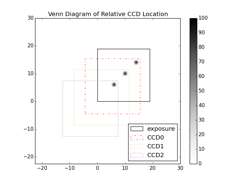
def ccdVennDiagram(exp, showImage=True, legendLocation='best'):
'''
Create a figure with the bounding boxes for each of the images which go into a coadd,
over-plotting the given exposure object.
exp [in] - (Exposure) The exposure object to plot, must be the product of a coadd
Optional:
showImage [in] - (Bool) Plot the data in exp in addition to just it`s bounding box, default True
LegendLocation [in] - (String) Matplotlib legend location code, can be: 'best', 'upper right',
'upper left', 'lower left', 'lower right', 'right', center left',
'center right', 'lower center', 'upper center', 'center'
'''
# Create the figure object
fig = plt.figure()
# Use all the built in matplotib line style attributes to create a list of the possible styles
linestyles = ['solid','dashed','dashdot','dotted']
colors = ['b','g','r','c','m','y','k']
# Calculate the cartisian product of the styles, and randomize the order, to help each CCD get
# it's own color
pcomb = np.random.permutation(list(itertools.product(colors, linestyles)))
# Filter out a black solid box, as that will be the style of the given exp object
pcomb = pcomb[((pcomb[:,0] == 'k') * (pcomb[:,1] == 'solid')) == False]
# Get the image properties
origin = lsst.afw.geom.PointD(exp.getXY0())
mainBox = exp.getBBox().getCorners()
# Plot the exposure
plt.gca().add_patch(patches.Rectangle((0,0),*list(mainBox[2]-mainBox[0]), fill=False, label="exposure"))
# Grab all of the CCDs that went into creating the exposure
ccds = exp.getInfo().getCoaddInputs().ccds
# Loop over and plot the extents of each ccd
for i,ccd in enumerate(ccds):
ccdBox = lsst.afw.geom.Box2D(ccd.getBBox())
ccdCorners = ccdBox.getCorners()
coaddCorners = [exp.getWcs().skyToPixel(ccd.getWcs().pixelToSky(point)) + \
(lsst.afw.geom.PointD() - origin) for point in ccdCorners]
plt.gca().add_patch(patches.Rectangle(coaddCorners[0], *list(coaddCorners[2]- coaddCorners[0]),
fill=False, color=pcomb[i][0], ls=pcomb[i][1], label="CCD{}".format(i)))
# If showImage is true, plot the data contained in exp as well as the boundrys
if showImage:
plt.imshow(exp.getMaskedImage().getArrays()[0], cmap='Greys', origin='lower')
plt.colorbar()
# Adjust plot parameters and plot
plt.gca().relim()
plt.gca().autoscale_view()
ylim = plt.gca().get_ylim()
xlim = plt.gca().get_xlim()
plt.gca().set_ylim(1.5*ylim[0], 1.5*ylim[1])
plt.gca().set_xlim(1.5*xlim[0], 1.5*xlim[1])
plt.legend(loc=legendLocation)
fig.canvas.draw()
1 Like
Hey @natelust that’s useful. What are the units on the $xy$ axes?
This will become a great tutorial (note to myself).
Another thought is that, for sky projections, wcsaxes is really awesome for plotting points and shapes with some sky coordinates into matplotlib. We (collectively) should establish patterns for plotting our Explosures with wcsaxes.
Looks like they are pixels in the coadd patch space.
The units of this are just in the pixel coordinates of the exposure. Where 0,0 corresponds to XY0 in the exposure object. Thus all the CCDs are just offsets of the location of the exposure object itself. It would be trivial to covert this to wcs axis as well, and maybe could be an option. I just make this as a simple way for me to see which CCDs contributed to which objects. It would also be great to update the function to label the legend with the butler info instead of just the string CCD+i, something with visit ccd or something.