A spotlight post for the third_obs family (from the v1.5 runs).
In this family, we implemented a strategy with the goal of adding a third visit for fields which had already acquired a pair of visits earlier in the night, in the WFD area (only). The variation across the family is “how much time is used for third visits?” – the comparison point would be against ‘baseline_v1.5_10yrs’, which is a similar strategy (same survey footprint and weighting – this is a traditional WFD and survey extensions in GP/NES/SCP).
- The third visits were only able to be acquired during the “Third” time before morning twilight – i.e. the third visits always happened at the end of the night.
- The third visit was always acquired in g, r, i, z or y . Which filter was used for this third visit would depend on what filter was already in the camera (we prefer not to change filters), but also on what the sky brightness was like in each filter at that time (these factors are the same as usual for any standard visits).
- A part of the sky would only be eligible for a visit in one of the g, r, i, z or y filters IF there was already at least two visits in any filter to that part of the sky and at least one visit in that same filter earlier in the night.
The amount of time between the earlier visits to the field and the third visit is not a factor in choosing where to observe – however, the standard basis function which drives visits toward the meridian (the m5 depth basis function) would tend to prefer visits to field which match the above criteria and are still relatively high in the sky – this means, in practice, the part of the sky that would get a third visit in the night would be that which was visible later in the night.
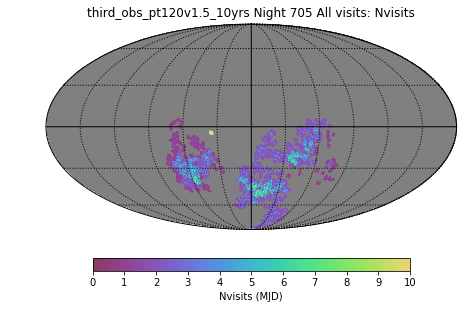
We can visualize this by looking at a night in a third_obs run which had a large number of third visits – third_obs_pt120v1.5_10yrs, night 654.
First: all of the visits obtained in the night. One of the aspects this illustrates is that we do sometimes observe parts of the sky more than twice, although most of the time we do not (and a lot, although not all, of the repeats are due to field overlaps – see “how many visits per night does a pointing receive?” and this Overlaps-NvisitsPerNight notebook). You can also see the DD field, the isolated dot. As an aside, a plot of the visits from the baseline survey on this same night looks very similar (it’s early in the survey).
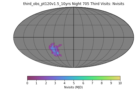
Then: the third visits from this night: (there were a total of 150, compared to 1011 visits throughout the night … on this particular night, there were 288 visits in u, 220 visits in g, 278 visits in r, 205 visits in i, and 20 visits in y … the moon was only 35% illuminated, or about 5 nights from new moon). So you can see they are in the later part of the night, at higher RA values. They are scheduled in a ‘blob’ in a similar fashion to earlier visits in the night outside of twilight. Some of these pointings are observed more than just once as well (giving us fourth or more visits per pointing) – this isn’t entirely unexpected in this run, given that we have 120 minutes devoted to obtaining thirds, but only a limited amount of sky will be desirable/available for this purpose. The runs with smaller amount of time (30 minutes or so) devoted to third visits show only single visits in the ‘third’ region.
Now, back to the amount of time expected to be devoted ‘third’ visits in each night and how to translate this from the run name, along with a comparison to approximately how much time was actually devoted to the third visits in each night. The “Third” time column represents how much time was programmed towards third visits per night (in minutes), along with a translation of that time into an approximate expectation of the fraction of visits (%), assuming an average 8 hour night, 80% of time spent on WFD (we only programmed third visits in the WFD area), and an average 77% open-shutter efficiency. The ‘Frac thirds’ column reports the approximate fraction of WFD-region visits that were actually used for third visits.
| RunName | “Third” time (%) | WFD Visits | WFD Visits (minus third) | Frac Thirds |
|---|---|---|---|---|
| baseline_v1.5_10yrs | 0 (0.00) | 1.85M | 1.85M | 0.00 |
| third_obs_pt15v1.5_10yrs | 15 (0.02) | 1.85M | 1.85M | 0.00 |
| third_obs_pt30v1.5_10yrs | 30 (0.04) | 1.85M | 1.82M | 0.02 |
| third_obs_pt45v1.5_10yrs | 45 (0.06) | 1.85M | 1.81M | 0.02 |
| third_obs_pt60v1.5_10yrs | 60 (0.08) | 1.86M | 1.76M | 0.05 |
| third_obs_pt90v1.5_10yrs | 90 (0.12) | 1.86M | 1.65M | 0.11 |
| third_obs_pt120v1.5_10yrs | 120 (0.15) | 1.87M | 1.56M | 0.16 |
Plotting this, for another view:
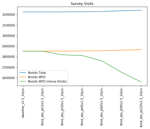
Generally speaking these behave as programmed – as more time is requested to be spent on ‘third’ visits, more time is used for this, and it roughly follows the fraction of time expected to be used for thirds. However, you can see a few nonlinearities, particularly with smaller fractions of time spent on thirds.
When there is only a small amount of third time programmed, the amount of time available before twilight is close to the amount of time typically used to cycle through a ‘blob’ (about 22 minutes to cover a blob once, 44 minutes to cover the blob twice to get pairs). The blobs executing in the main part of the night queue up their first round and then execute the follow-up pair visit without allowing interruption from these ‘third’ visits – so it becomes a matter of chance related to how long the usable night is, when standard pair blobs started executing, and how fast they finished, as to whether and how much time is available for third visits. Once the third visit blob starts executing, third visits will continue until morning twilight starts … but the amount of time actually available for this will vary somewhat, and when the time requested for thirds is small, this creates more ‘noise’ in how much is actually used. This explains why the 15, 30 and 45 minute thirds simulations all fall short of the amount of time requested for third visits (and thirds with only 15 minutes available actually fail to execute at all in a meaningful way).
So there are useful things with this family of runs – some parts of the sky will have boosted numbers of visits per night (particularly in the same filter). However, there are also some complications in the impacts these runs may have on metrics:
- on a normal night, any point in the sky often receives more than just a pair of visits to a field, although a lot of this is due to field overlap and so may not include large contiguous areas
- for small amounts of time devoted to third visits, the amount of time actually available will vary in a slightly non-linear way (but the third visit region will likely consist of a single visit, which is constrained to be in a filter already used in the night)
- for large amounts of time devoted to third visits, the amount of time available is likely to match the desired amount closely, but the third visit region is likely to acquire more than just a single additional visit.
- for any set of visits which are acquired in pairs in standard blob operations (the middle of the night standard pattern), the pair separation will be very close to the desired time. For the third visit, there is no constraint on time separation from that pair, except that it cannot be larger than the total amount of time per night devoted to thirds. (this could be a boost to some metrics, but it depends on the science requirements).