The first question the SCOC is asking everyone to address in the Cadence Notes is:
Q1: Are there any science drivers that would strongly argue for, or against, increasing the WFD footprint from 18,000 sq. deg. to 20,000 sq.deg.? Note that the resulting number of visits per pointing would drop by about 10%. If available, please mention specific simulated cadences, and specific metrics, that support your answer.
At the very highest level, this is simply asking which is more important for your science - more visits per pointing or more area (assuming a limit on the total number of visits)? In answering, it is useful to consider if your science degrades or improves more gently with area vs. with the number of visits per pointing, or if there are any points at which further changes would ‘break’ your science (such as if you suddenly did not have enough visits in a given time interval to detect or classify transient or moving objects). However, the SCOC is not asking this in a vacuum and so have supplied a specific range of area, and we have some simulations that should help address the question in qualitative ways.
The SurveyFootprints-NvisitsVsArea notebook attempts to help identify simulations which cover this range of area in various footprints. It’s worth noting that even 20,000 sq degrees doesn’t stretch to cover all of the sky that everyone would be interested in; so an important part of this question is where that area is distributed.
Because the vast majority of our simulations are aimed at covering close to 18k sq degrees, I took some pains to try to be able to include all of the existing simulations and try to evaluate them on a somewhat equal footing. The major difference for this particular analysis is the overall number of visits and the mean number of visits per pointing; for runs with 1x30s visits, we can obtain about 9% more visits than we do for runs with 2x15s visits (which is and will be the default until we can test the camera on-sky, at a minimum). To try to make all of the runs comparable in this particular evaluation, I adjusted the result of visit count metrics in 1x30s runs downward by a factor of 0.922. In order to measure how much area included in the ‘WFD’ in each simulation, I just looked at how much of the sky was covered to at least 750 visits (in 2x15s runs; 813 visits in 1x30s runs) in the simulation. I used 750 visits as the cutoff, as this is the ‘minimum’ requirement for visits per pointing in the WFD in the Science Requirements Document; we typically measure the area that receives at least 825 visits in the standard MAF outputs, so this is similar but with a different threshold.
I could then compare the median number of visits per pointing vs. the area covered in the WFD for each survey, as well as evaluate approximately what fraction of the total visits were used to cover this area. I took a set of simulations which cover the sky to varying amounts of area above 18k sq deg with various footprints, and come up with this set of runs that may be interesting comparison points:
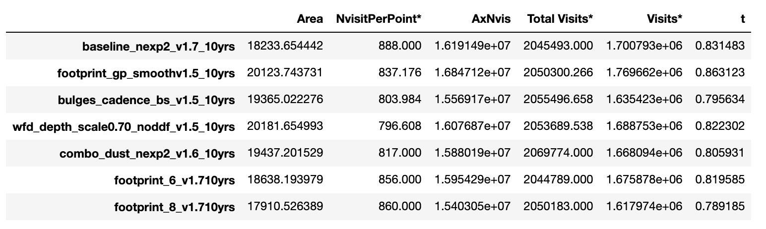
The notebook linked above has plots showing the footprint for each of these runs.
Here is a plot of the mean number of visits per pointing vs the WFD area for these simulations:
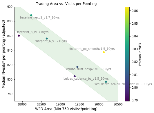
Most of these runs devote approximately 80-83% of the total visits to the WFD area, which is shown by the green stripe in the plot above.
It is likely that we cannot count on devoting significantly more than this fraction of time to the WFD. In the current survey strategy we typically use 5% for DDFs, at least 4% for other parts of the sky outside the WFD (the placement of the WFD strongly influences this fraction, and the required number of visits may be higher … or slightly lower), 1-2% should be saved for mini-minisurveys and ToOs, and we are currently starting to attempt to hold on the order of 5-8% to boost the number of visits within the WFD as ‘contingency’ in case of excessively bad weather or mechanical failures (which is not reflected in the number of visits per pointing in the above plot, as those visits were typically directed to other mini-survey areas).