Survey Strategy and Solar System Science

[ljones (Lynne Jones)]

Some thoughts and metrics related to the survey strategy and solar system science.

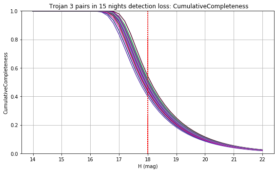
Context: general solar system science metrics include discovery metrics (with various discovery criteria) and characterization metrics (ie. how many colors for objects can we measure, and can we determine a light curve or even shape measurement from the lightcurve). The most important metric is discovery; if we can’t find the objects, then we can’t do anything else with them (or follow them up at other observatories). Secondary metrics are all of the characterization metrics. There are multiple populations of small bodies throughout the solar system, which move with different apparent velocities and cover varying amount of the sky (generally centered on the ecliptic, but some more widely distributed than others).
As such, survey strategy can have different effects on different populations, even when considering just one metric. Secondary metrics can also be important, especially if the primary discovery metric isn’t a strong differentiator between strategies.

With that, we can look at various aspects of the survey strategy.

First up - intranight strategy
The relevant simulations here include visits = 2x15s snaps or visits = 1x30s snap, whether we have single visits per night, double visits, or triples (for some fraction of each night).
The relevant simulations (due to an oversight on the project side) include runs from FBS 1.4 and FBS 1.5 … the metric outputs for each run are normalized by the relevant baseline_vX_10yrs output.
The list of runs included for consideration are:

 ['nopairs_v1.4_10yrs', 
'baseline_2snaps_v1.5_10yrs', 
 'baseline_v1.5_10yrs', 
'baseline_v1.4_10yrs',
 'baseline_samefilt_v1.5_10yrs',
 'third_obs_pt15v1.5_10yrs', 
 'third_obs_pt30v1.5_10yrs', 
 'third_obs_pt45v1.5_10yrs', 
 'third_obs_pt60v1.5_10yrs', 
 'third_obs_pt90v1.5_10yrs', 
 'third_obs_pt120v1.5_10yrs']

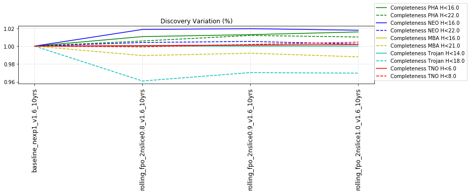
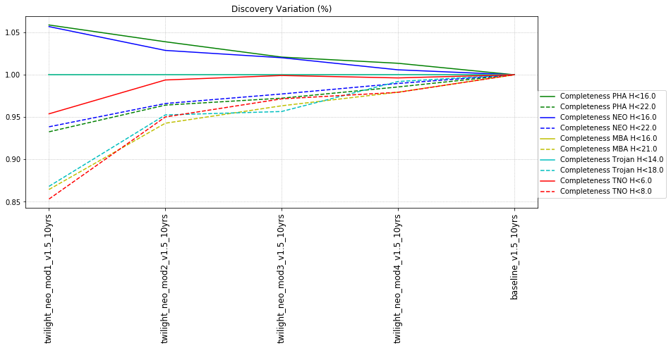
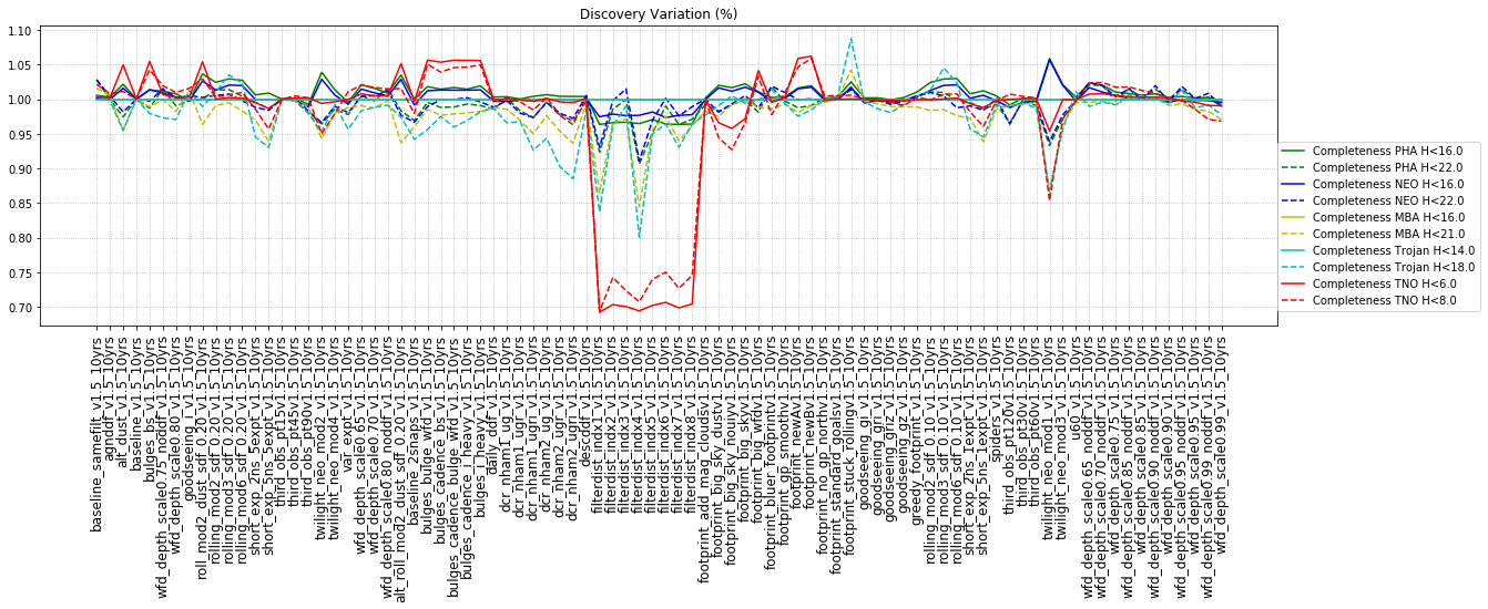
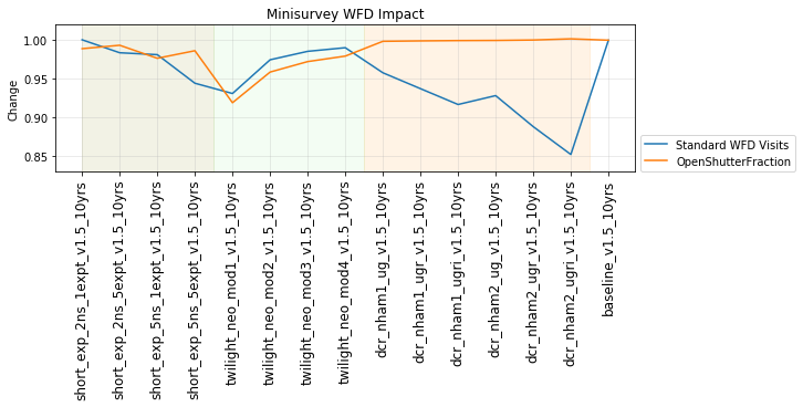
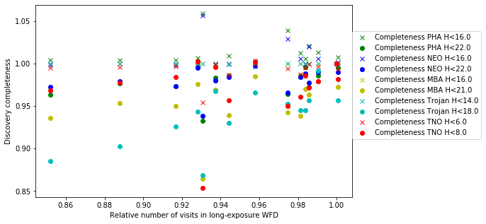
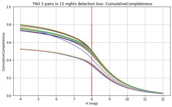
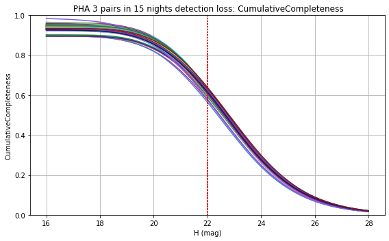
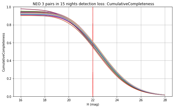
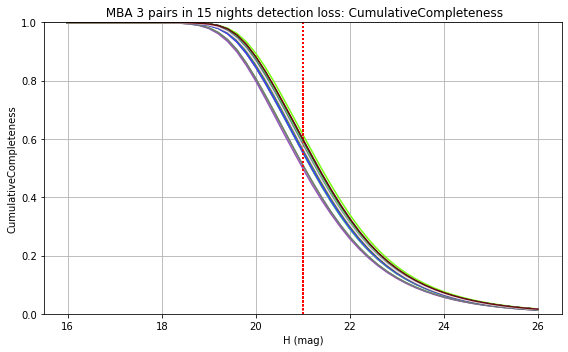
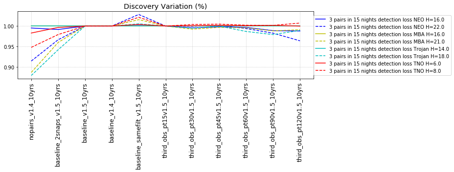
The punchline is the following plot, showing the discovery completeness at bright and 50% values, for various populations, across all of these runs.

It may be surprising that the ‘no pairs’ simulation results in any objects being found at all - that we do find any means that fields have not-insignificant overlaps within a night, that sometimes objects move between fields, and that sometimes we take pairs of visits in a night anyway.
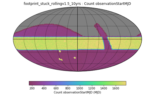
This can be seen in the intranight histogram as well … no pairs and standard baseline histograms below, which show that the number of repeat visits within a night drops significantly for the no-pairs simulation, but not to 0.


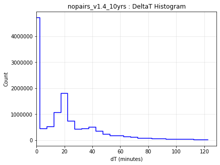
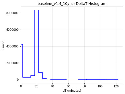
It should be noted that the existence of overlaps of visits in the ‘no-pairs’ state is fragile … if the scheduler algorithm was changed to reduce overlaps, then these would likely disappear.

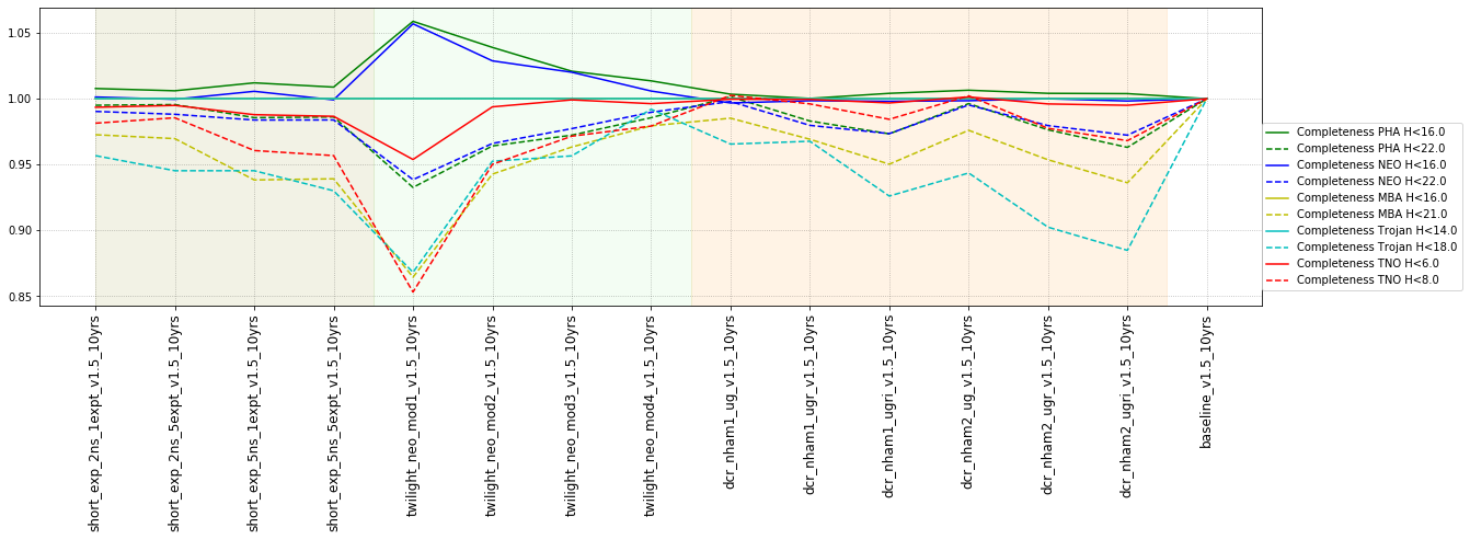
This shows that the favored strategy would be taking pairs of visits, in the same filter within the night (about a 3% improvement in the discovery fraction of NEO and PHAs). Strongly disfavored strategies would be single visits per night (an over 10% hit for main belt asteroids), due to the requirement of two observations per night for MOPS linking. The 2x15s strategy (2snaps) vs. 1s30s strategy (1snap per visit) involves about a 5% decrease in completeness for Trojan asteroids, with varying decreases among other populations – this is generally linked to the overall fewer number of visits possible when doing 2snaps vs. 1. Observing with a triple visit near the end of the night is not a significant issue until the amount of time devoted to triples is large (the pt90 and pt120 runs), at which point it can result in about 4% fewer NEOs being discovered. This is most likely due to the decreased amount of sky observed in each night.

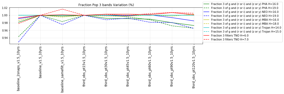
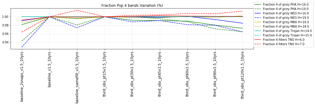
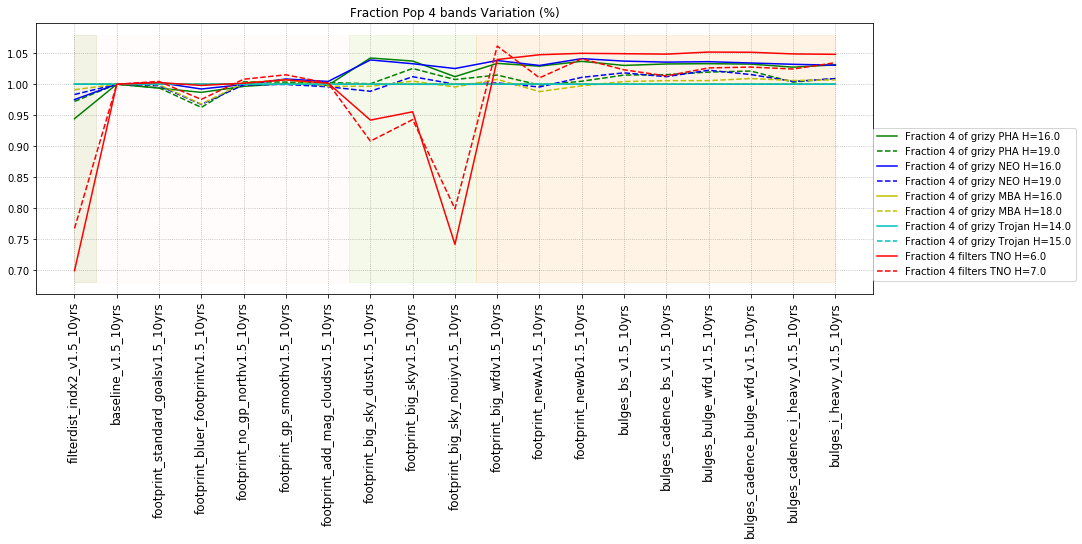
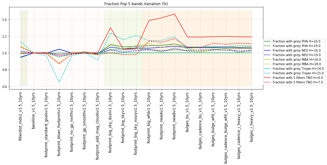
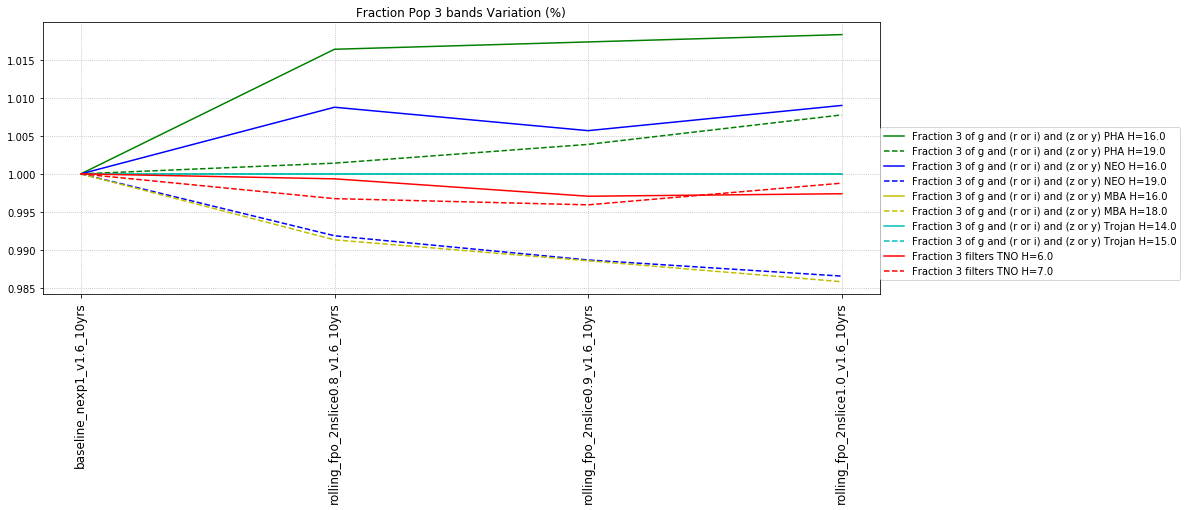
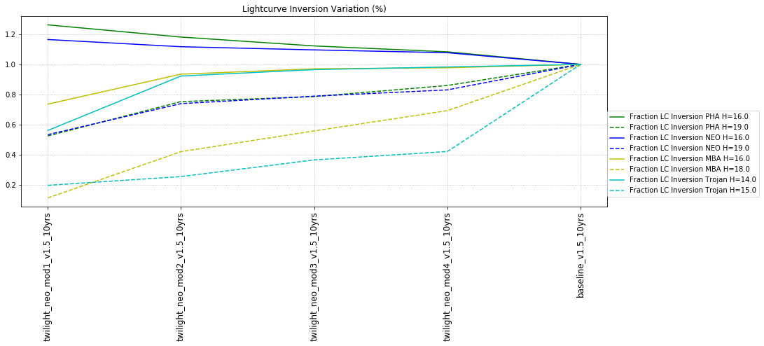
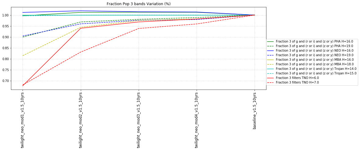
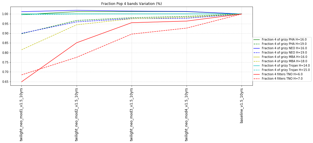
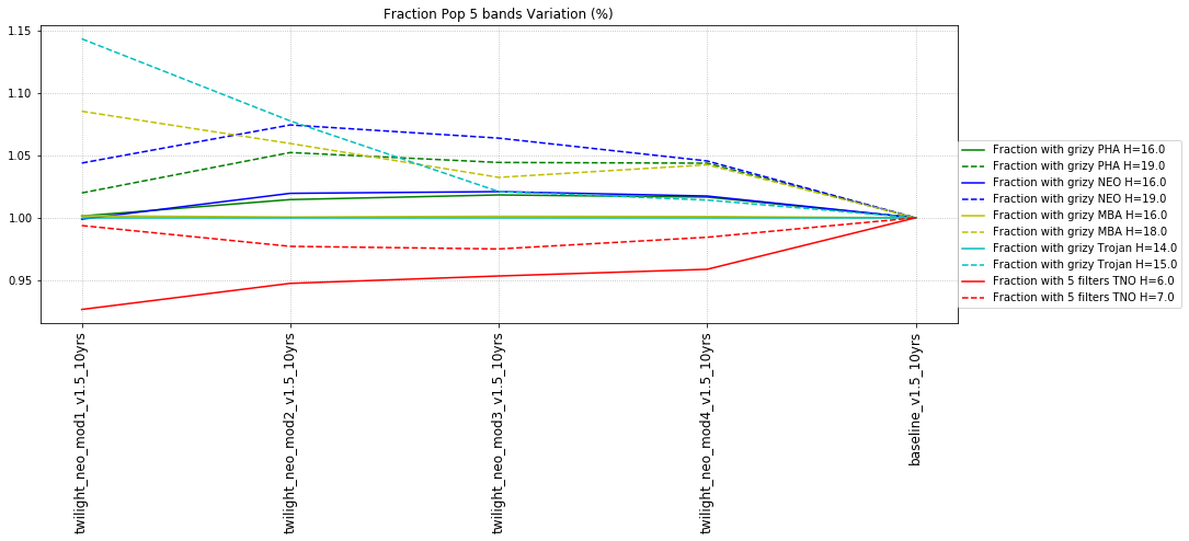
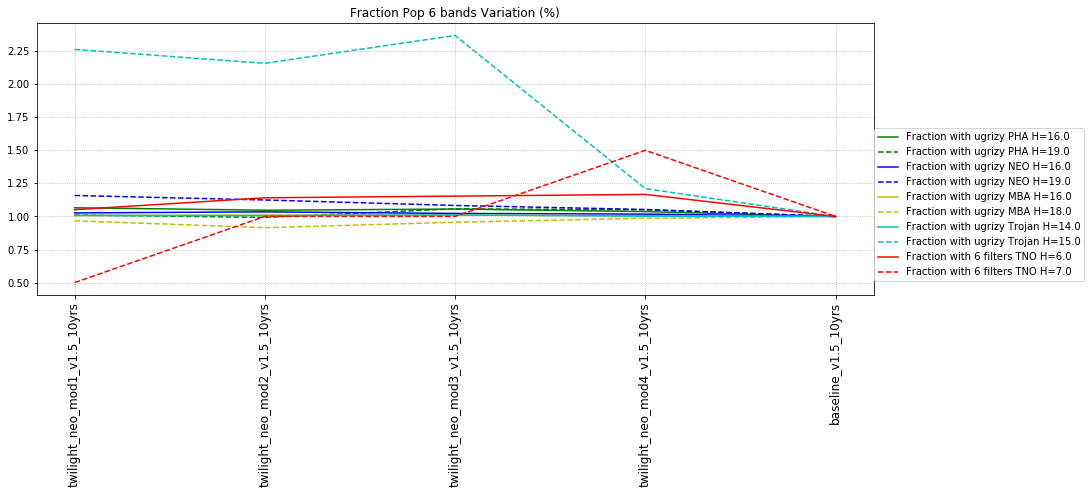
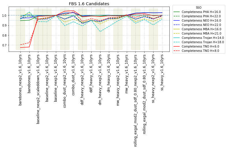
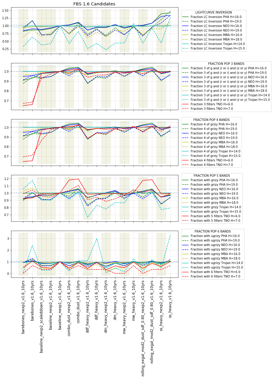
It’s worth noting that observing each pair in the same filter, while it has a benefit for discovery, has a small cost for characterization, at least when looking at the number of objects which can be measured in 4 colors (primarily for Jovian Trojans). Here are the characterization metrics: there is a difference between outer solar system (TNO) and inner solar system (PHA, NEO, MBA, Trojan) metrics here.
Inner solar system metrics for colors look specifically for the fraction of the population with:

• Three of either g and (r or i) and (z or y) – i.e. obtain 2 colors g-r or g-i PLUS g-z or g-y
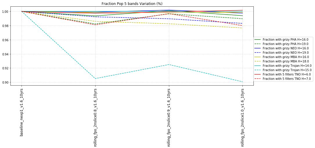
• Any 4 different filters (from grizy). i.e. 3 colors = g-r, r-i, i-z, OR r-i, i-z, z-y.
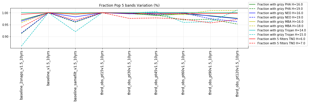
• All 5 from grizy. i.e. 4 colors = g-r, r-i, i-z, z-y.
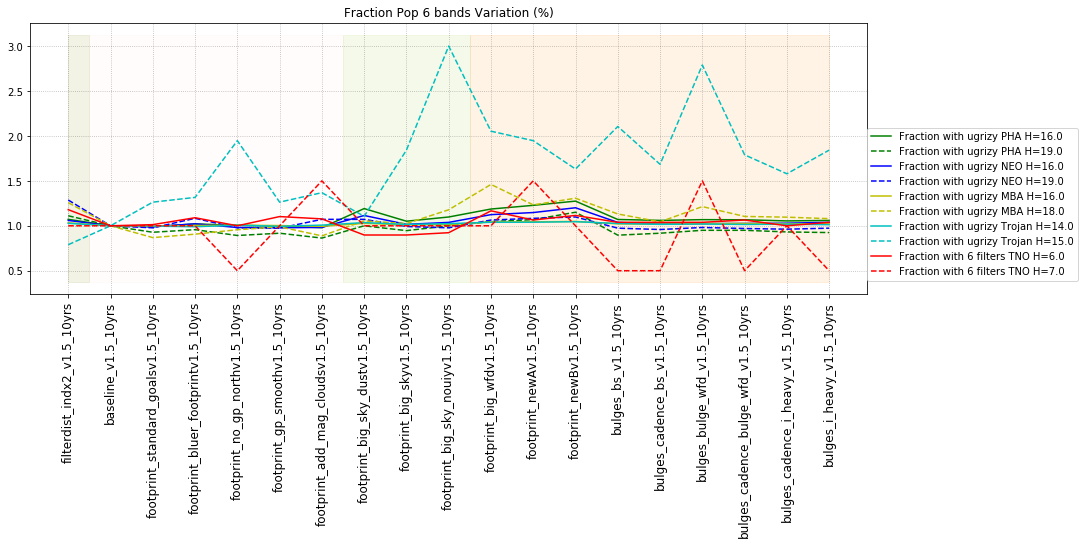
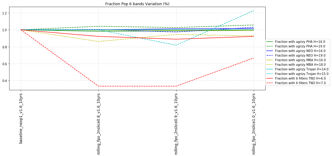
• All 6 filters (ugrizy) – best possible! add u-g color
  To decide if a filter is ‘acceptable for color determination’, the metric calculates the sum of a snr-weighted number of visits and compares that to a threshold value. For example, in the standard configuration, either 41 visits with a snr of 5 OR 11 visits with a SNR of 20 would need to be acquired to count as a detection in a single band (SNR values higher than 20 still require at least 11 visits).

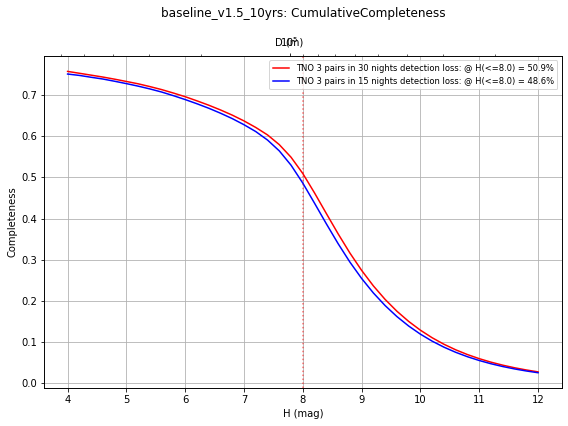
Outer solar system metrics for colors look for the fraction of the population with:

• enough visits in a single band for a lightcurve (default 30 visits) (1 band)
• enough visits in a primary band for a lightcurve, plus additional visits (default 20) in another band to measure a color (2 bands = 1 color)
• additional visits (20) in additional bands for more colors (3 bands = 2 colors, etc.)
  So, less specific colors and a slightly different way to count towards a color.

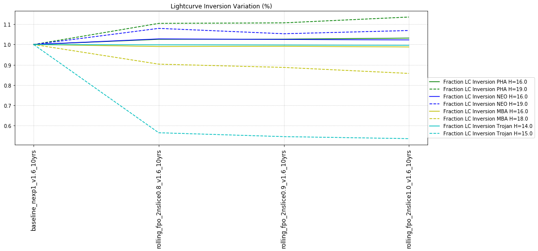
The inner solar system also has an additional metric for lightcurve inversion. This metric likewise looks for a certain number of SNR-weighted observations (the default would be equivalent to 1000 observations at SNR of 5 or 50 at SNR of 100 or 250 at SNR of 20). It then adds more requirements on the phase angles of the observations – the phase coverage must be more than 5 degrees, the range of ecliptic longitudes has to be more than 90 degrees, and the absolute deviation of the ecliptic longitude coverage has to be more than 1/8 of the coverage range.

[ljones (Lynne Jones)]

Next: footprint

The footprint generally means “what does the survey footprint look like”, and in particular, tends to refer to what does the WFD or high-numbers-of-visits portion of the footprint look like. There can be variations in the filter distribution, but primarily we’ve investigated what part of the sky the WFD (or which part of the sky tends to get 500-1200 visits) portion of the survey looks like.

The relevant footprint runs can all be pulled from the FBS 1.5 release. The sets of runs with relevant information include the “footprint” series, the “bulge” series (because these include heavy coverage through the galactic plane in various ways), and the “filter_dist” series (because these include variations in filter coverage, but also - importantly - they feature a restricted survey area that includes no visits in the North Ecliptic Spur). The specific runs are:

['filterdist_indx2_v1.5_10yrs',
 'baseline_v1.5_10yrs',
 'footprint_standard_goalsv1.5_10yrs',
 'footprint_bluer_footprintv1.5_10yrs',
 'footprint_no_gp_northv1.5_10yrs',
 'footprint_gp_smoothv1.5_10yrs',
 'footprint_add_mag_cloudsv1.5_10yrs',
 'footprint_big_sky_dustv1.5_10yrs',
 'footprint_big_skyv1.5_10yrs',
 'footprint_big_sky_nouiyv1.5_10yrs',
 'footprint_big_wfdv1.5_10yrs',
 'footprint_newAv1.5_10yrs',
 'footprint_newBv1.5_10yrs',
 'bulges_bs_v1.5_10yrs',
 'bulges_cadence_bs_v1.5_10yrs',
 'bulges_bulge_wfd_v1.5_10yrs',
 'bulges_cadence_bulge_wfd_v1.5_10yrs',
 'bulges_cadence_i_heavy_v1.5_10yrs',
 'bulges_i_heavy_v1.5_10yrs']

To visualize the difference in these footprints, here are plots of the distribution of total visits for each of the above runs (using the same scale for each simulation):

Limited WFD footprint types …

• all of the filterdist runs have this same map, which covers a declination region similar to the standard survey WFD, with no variation across the galactic plane, and no NES or SCP coverage. The variations on filterdist have different filter distributions.
  
  

Standard survey variations

• footprint_standard_goals is the same as baseline_v1.5, basically. This is the old standard survey footprint. The footprint_bluer_footprint survey uses this same map, however it has a bluer filter distribution (more u/g, less z/y).
  
  
• footprint_no_ gp_north is similar to the standard survey, but removes the northern extension of the galactic plane (GP).
  
  
• footprint_add_mag_clouds adds an extension to the standard footprint at the Mag Clouds
  
  
• footprint_gp_smooth covers the (large) galactic plane to the same limits as the standard WFD. The rest of the footprint is similar to standard.
  
  

Extended N/S WFD coverage

• footprint_big_sky_dust uses an extended N/S region for the WFD (going about 10 degrees further north and south), with the galactic plane boundaries delinated by dust extinction. There is extended coverage with fewer visits to the north, but no SCP or galactic plane coverage.
  
  
• footprint_bigsky uses a similar extended N/S region for the WFD, with the galactic plane boundaries defined by a galactic latitude (=20deg) only. footprint_bigsky_nouiy is similar, but without u, i or y bands. Like in the footprint_bigsky_dust, there is extended coverage with fewer visits to the north, but no SCP or galactic plane coverage.
  
  
• footprint_bigwfd is sort of a hybrid between the big sky and the standard survey; it has an extended WFD region, going further north than in the big sky but not as far south. This footprint includes SCP and GP coverage, with a small extension for the NES.
  
  
• footprint_newA includes an extended N/S WFD (big sky style), with galactic plane region defined by galactic latitutde (l=20). The bulge direction is covered to slightly fewer visits than the full WFD; the anti-center is covered to normal WFD depths. The SCP and NES (and extended northern coverage) is included, to a more limited depth. The WFD region only achieves about 771 visits per pointing.
  
  
• footprint_newB is similar to footprint_newA, but the galactic anti-center is covered to much fewer visits in an attempt to redistribute these into WFD and add to NES. The WFD region here achieves a median of 842 visits per pointing.
  
  
• bulges_bs and bulges_cadence_bs use the same footprint map, although with different timing for the galactic plane coverage. Note that the WFD is extended N/S beyond the ‘standard’ footprint, so this is like the ‘big sky’ footprint, but with bulge, northern, and SCP coverage.
  
  
• bulges_bulge_wfd and bulges_cadence_bulge_wfd, and bulges_i_heavy and bulges_i_heavy_cadence all use this survey footprint map, although with different timings and filter distributions. Note that it is similar to the big sky basis, but with galactic plane and SCP coverage, and these variations also have a band of WFD-level coverage through the galactic bulge.
  
  

In terms of solar system object discoveries, we might expect the footprint to be a significant contributor. This is true particularly for TNOs, as they move very slowly across the sky. NEOs cover large amounts of the sky, thus are less sensitive to footprints. The MBAs are similar to the NEOs, although more constrained toward the ecliptic plane. The Trojan asteroids are also sensitive to footprint, as they are concentrated into limited sky locations due to their resonant nature.

We can again look at the discovery completeness at bright and 50% values, for various populations, across these footprint-related runs (organized by type of footprint):

It’s clear that the filter_dist* run, where the NES was not covered, have a severe impact on TNO discovery (-30%). (the other filter_dist runs are similar, though not included in the plot above to reduce clutter). None of these filter_dist runs improve solar system object discovery, even though the WFD region will have more visits within its footprint.

In these runs, the trend for most populations improves from the filter_dist family [olive], then remains fairly constant through variations on the standard baseline footprint (though the filter distribution in ‘bluer footprint’ impacts various populations somewhat) [light pink], decreases through the big_sky runs (which did not cover the galactic plane region) [light green], and then increases again at least for the brightest members of each population with big sky footprints that have heavier coverage of the GP plus NES – these wider area footprints have fewer visits per pointing in the WFD, in general.

For TNOs, the winner is clearly any simulation that has the widest sky coverage – including the GP. It’s worth noting that difference imaging for TNO discovery may be difficult near the galactic plane - however, transient and variable studies will also rely on this difference imaging, so it may be reasonable to assume it will work to some level (and thus benefit TNO discovery to some level, even if not as far as implied in these trends).

For other populations, the variations across footprints are not quite as strong – on the order of 3% instead of up to 5% (discounting the filter_dist runs for TNOs). The bright PHA and NEO population completeness is better for the ‘big-sky’ style runs (both big_sky* and the bulges*related variants) … presumably due to sky coverage again. However, the fainter PHA and NEO population completeness falls slightly in these big_sky style surveys, likely due to the fewer number of visits per pointing (as these smaller objects reach bright apparent magnitudes for a shorter amount of time, you have to have more visits to ‘catch’ them).

Checking in with characterization, we find more ties with filter distribution across the footprint than the footprint map itself (this is more visible across the filter_dist runs), although the increase in TNO observations in the big_sky style runs is again visible, with a huge increase with newB (which has additional observations through the NES, in comparison to most of the other big_sky footprints).

[ljones (Lynne Jones)]

Next: rolling cadence

Update – so, we found a problem with the rolling cadence simulations with more than 2 bands … they weren’t really ‘rolling’ as hard as we thought they would, and in fact, weren’t really up to it at all. We’re re-running these simulations with some fixes, so let’s come back to this question a bit later.

For now: here’s two-band rolling (some slightly different versions, although I don’t believe they are significantly different as we’d hoped) vs. not rolling. I believe these should be correct, however it’s reasonable to wait for confirmation from the new set of rolling cadence runs we’re working on.

The FBS 1.6 ‘rolling_fpo’ runs (rolling footprint from FBS 1.6) have 1x30s visits, so should be compared against the FBS 1.6 baseline_1nexp_v1.6_10yrs run (which also uses the new footprint).
These runs include:

['rolling_fpo_2nslice0.8_v1.6_10yrs',
 'rolling_fpo_2nslice0.9_v1.6_10yrs',
 'rolling_fpo_2nslice1.0_v1.6_10yrs',
 'baseline_nexp1_v1.6_10yrs']

We’ll have to wait to see the new rolling cadence runs, but it’s interesting to think about why the two-dec band rolling cadence would make it slightly easier to find big objects but sometimes harder to find the smaller objects (in the Trojans and MBAs). The difference is only between 51% completeness (in the baseline) and 49% completeness (in the rolling cadence) for Trojans; this is possibly still within the statistical variation range, so this is only a small difference, I’d say.

Once again checking in with characterization -

[ljones (Lynne Jones)]

Next: twilight NEO surveys

To evaluate the effect of a targeted NEO twilight survey, we look at the ‘twilight_neo_mod[1,2,3,4]_v1.5_10yrs’ series:

['twilight_neo_mod1_v1.5_10yrs',
 'twilight_neo_mod2_v1.5_10yrs',
 'twilight_neo_mod3_v1.5_10yrs',
 'twilight_neo_mod4_v1.5_10yrs',
 'baseline_v1.5_10yrs']

In each of these simulations, an additional twilight time NEO-targeted survey was added. The NEO-targeted visits consist of 1 second exposures in r, i, or z band (bandpass used depends on which filter was previously in use in the camera, which means it is loosely tied to lunar phase but also survey progress). For each night where the twilight survey was triggered, there were attempted observations in the evening twilight and morning twilight, typically about 440 visits per night. The observations within a given night required triplets for each field pointing. The fields chosen for the NEO survey were within 40 degrees of the ecliptic, at high airmasses toward the sun.
The “modX” indicates how frequently the twilight_survey was triggered; 1 = every night*, 2 = every other night*, 3 = every third night*, 4 = every fourth night*.
(*where possible … there were some nights where weather would have not permitted visits in one or both of the twilight periods, etc.)

Number of visits per night for the twilight survey, in the twilight_neo_mod1 and twilight_neo_mod4 simulations:


and statistics (mean/median/percentiles) on the number of twilight NEO survey visits in each night and the number of nights the twilight survey was executed (“Count”).

Sky coverage patterns for an individual night in the twilight_neo surveys (night chosen based on the 'first night that had more than 500 visits in the twilight_neo survey):

After the full ten years of the survey, the sky coverage included in the twilight survey looks like:

After this time, the field altitude and solar elongation histograms for the twilight_neo survey fields looks (similar for each different simulation)

Ok, description of the twilight survey characteristics out of the way - what was the impact?

In general it looks like a win or slight neutral for the bright/large end of the populations but a loss at the faint end of the populations, with this effect being strongest for the case when the twilight_neo survey executed every possible night (mod1). When the twilight survey exectued every night, large NEOs and PHAs showed a ~5% increase in completeness, but small NEOs and PHAs had a ~6% loss in completeness. Other fainter populations had even stronger losses - smaller Trojans and TNOs lost 15% in completeness. This can be understood when we look at the overall number of standard (longer exposure) visits in the WFD in each of these twilight_neo cases compared to the baseline:

The twilight time taken by executing the twilight NEO survey appears to be necessary for standard operations. In the case of twilight_neo_mod1, the number of visits for “other purposes” drops by 10% – a significant loss, that is likely the cause of the decreased completeness for smaller/faint objects (which don’t benefit so much from the 1second visits in the twilight neo survey).
(Edit to add here, as well as below - ‘twilight’ in this case involves observations starting as 12 degree twilight. This time is used for both the start of regular operations and the start of ‘twilight’ survey observations).

Again checking on the effect on characterization:

[ljones (Lynne Jones)]

Then: Any other effects (from other survey strategy choices)

The families of simulations above cover the most obvious questions related to solar system science. It’s worth asking if any of the other simulations created for other purposes (such as adding high airmass visits for DCR measurement, or adding short exposures over the sky for bright star measurements) impact solar system objects significantly, either in a positive or negative way.

If we look at all of the runs available in FBS 1.5, we get a very crowded plot …

but you can see the clear impact of the lack of the NES in the filter_dist series, the variations coming from the footprint and bulges series, as well as the twilight_neo family. These are the most obvious variations, and we’ve already discussed those above.

Pulling out those runs that we already covered:

Looking at some subsets of these:

The WFD-depth series (to the right in the plot above) are a family of simulations which varied the weight given to the WFD region, looking at some metrics related to SRD quantities. Increasing the amount of time spent on the WFD increases the number of visits per pointing inside the WFD; however, it is also means spending correspondingly less time on the mini-surveys such as the NES and the GP. There isn’t a huge amount of variation across these options, but to me it looks like an indication that solar system discovery depends not only the number of visits in the WFD, but also on the area covered over the sky (a viewpoint reinforced by the footprint and bulges series), and that the areas outside the traditional WFD footprint are important.

The other story I see there is in the dcr_[x] family of runs, as well as the short_exp[x] family. The DCR family added high airmass visits (in singles) a few times a year, while the short_exp family added short exposures (in singles) over the sky; neither types of visits are particularly suitable for discovering solar system objects, although this varies to a greater or lesser extent. As more time is spent on these kinds of observations, less time is available for standard visits which lend themselves to solar system discovery and the lower the completeness for solar system objects.

Putting these trends together:

It’s worth commenting on the footprint_stuck_rolling run, which stands out as neutral or an improvement for completeness in all solar system populations. This is somewhat surprising, as this simulation was intended as a test case for ‘breaking’ science: it is a rolling cadence, where the ‘rolling’ portion of the sky doesn’t actually swap as intended. The final footprint looks like

While most populations have neutral or slightly better than baseline results with this simulation, the small Trojan population enjoys an 8% boost.

[RobSeaman]

@ljones

The twilight time taken by executing the twilight NEO survey appears to be necessary for standard operations.

The notion that what is called “twilight time” might be subsumed into standard operations was perhaps not clear at the time the white papers were written, rather the notion for this variation of a twilight survey and perhaps others was to make use of time before the WFD survey starts and after it ends each night. What was the definition here of when twilight begins and ends? Presumably no simulation of the effect of mega-constellations was included?

@ljones

win or slight neutral for the bright/large end of the populations but a loss at the faint end

Presumably bright means H≤16.0 and faint H≤22.0 for NEOs? If the “most important metric is discovery” these detection statistics may need to be weighted by the 90+ % (perhaps 99%) completion for H≤16.0 at the start of the Survey and ~43% completion for H≤22 at the start. Many detections of all of these objects will not represent new discoveries. Have any of the simulations tagged the known populations? This may have a significant effect on near-sun discoveries since Rubin’s significantly fainter limiting magnitude is anticipated to offer a disproportionate benefit, which is to say that the trade-off may be between discoveries near-sun and re-detections near opposition.

[ljones (Lynne Jones)]

Hi @RobSeaman,

Yes, I think the concept of ‘twilight time’ was maybe not well communicated at the time of the white paper call. In the twilight_neo simulations, we start observations at a sun altitude of -12 deg (astronomical twilight) and in the standard simulations we did also. At the time of writing the call for white papers, we thought this 12-18 degree twilight time was not required for WFD visits … with the more pessimistic weather conditions we use now, and the number of other minisurveys in play, we do now need this time to meet WFD requirements.

I think we could look into doing the twilight survey during nautical twilight, but it wasn’t clear (to me anyway) whether that was what people were talking about.

No, we are not including the effects of mega-constellations of satellites. I suspect if we have a true mega-constellation, it will not be worth doing twilight surveys for NEOs anyway, but I could very well be wrong. We don’t know enough about it yet, but I am a bit pessimistic perhaps.

I did not include ‘previously known’ objects in the metric … it’s something we could do. If most of the H=16 objects are known at the start of the survey, I’m not sure that I follow that the twilight surveys would be helpful … adding the twilight surveys decreases completeness for the H=22 NEOs.

[ljones (Lynne Jones)]

I got some questions / requests for clarification via email, which I will answer here for everyone:

1x30s vs. 2x15s visits – where are these? These two kinds of simulations are in the 'Intranight strategy" in the first post. The ‘baseline_2snaps’ runs have 2x15s visits, but everything else has 1x30s visits. In terms of the overall number of visits in the simulation, going from 2x15s visits to 1x30s visits lets us cram in about 7% more observations overall (due to smaller overheads from the readout and shutter open/close). But the impact on population completeness when going from 2x15s (the current default still) to 1x30s is smaller: (these are % changes in overall completeness)

3 pairs in 15 nights detection loss NEO H=16.0       0.850044
3 pairs in 15 nights detection loss NEO H=22.0       3.458009
3 pairs in 15 nights detection loss MBA H=16.0       0.000000
3 pairs in 15 nights detection loss MBA H=21.0       4.170132
3 pairs in 15 nights detection loss Trojan H=14.0    0.000000
3 pairs in 15 nights detection loss Trojan H=18.0    6.143443
3 pairs in 15 nights detection loss TNO H=4.0        0.240449
3 pairs in 15 nights detection loss TNO H=8.0        2.117227

(with base completeness levels in the 2x15s simulation of

3 pairs in 15 nights detection loss NEO H=16.0        91.760000
3 pairs in 15 nights detection loss NEO H=22.0        58.046157
3 pairs in 15 nights detection loss MBA H=16.0       100.000000
3 pairs in 15 nights detection loss MBA H=21.0        56.690961
3 pairs in 15 nights detection loss Trojan H=14.0    100.000000
3 pairs in 15 nights detection loss Trojan H=18.0     47.059684
3 pairs in 15 nights detection loss TNO H=4.0         74.860000
3 pairs in 15 nights detection loss TNO H=8.0         47.579377

At the bright end, we see small effects while at the faint end, the effects are larger. This reflects the fact that large/bright objects get more opportunities for discovery anyway, so are less sensitive to having more observations in the survey.

What does the FracPop5 metric do? Sorry, I should have clarified this. There are a number of characterization metrics run for each population – the inner solar system (everything out to TNOs) and the outer solar system (the TNOs) have slightly different metrics for these. You can see the full results for each simulation at http://astro-lsst-01.astro.washington.edu:8081/ (for the FBS 1.5 runs).
For the outer solar system, characterization is evaluated using the LightcurveColor_OuterMetric which looks for a primary bandpass that has enough visits to determine a lightcurve, and then secondary bandpasses that would have enough supplemental observations to determine a color. The result of the metric tells you how many bandpasses it could have a color (with another bandpass having a lightcurve) in – for the outer solar system then “FracPop5” = the fraction of the population which had a lightcurve in one bandpass and then four other bandpasses with enough for color information … yielding four colors and a lightcurve.
For the inner solar system, characterization is evaluated with the Color_AsteroidMetric for colors, and separately for lightcurve inversion potential with LightcurveInversion_AsteroidMetric. The asteroid color metric looks for enough SNR-weighted visits in various bandpasses to establish a color; the colors are required to be in particular filters. For the inner solar system populations, ‘FracPop5’ indicates that the asteroid was observed with enough visits in grizy to obtain colors with those bandpasses.

There were some more questions about the twilight survey, but I think those are handled above.

I realize the plots are somewhat hard to read. I did a relatively quick job plotting these using pandas plotting functions directly, so the colors and linestyles aren’t assigned … I can work on it, but you can also access all of this information directly (see CSV files for discovery and characterization for each simulation release at https://epyc.astro.washington.edu/~lynnej/opsim_downloads/ (*csv), the list of runs in each subset of simulations is in the thread above, and you can recreate this work using the notebooks on the epyc Jupyterhub server (which SSSC members have access to) - they are the *ipynb files in the common/2020_June directory (Intra-night Strategy.ipynb, Footprint Strategy.ipynb, Rolling Strategy.ipynb, and Twilight NEO surveys.ipynb).

[mschwamb (Meg Schwamb)]

Is plotting H=4 TNOs diagnostic for the Kuiper belt/TransNeptunian region? H=4 is the dividing line for dwarf planets. Would plotting H=6 TNOs be more reflective of TNO discovery statistics or does it look the same as H=8?

[ljones (Lynne Jones)]

Good point, in general H=4 and H=6 would look the same; H=8 show more variation because it is in the area of the completeness curve that is dropping more rapidly. For TNOs completeness does not drop as fast as it does for other populations. I suppose there may be some simulations where completeness drops faster or earlier if the images are shallower, so using H=6 might be a good change.
The completeness curves look like this:

and for all of the 1.5 simulations they have similar ratios at H=4 and H=6 …

and for the other populations I was just using the brightest objects so used H=4 here.
I could see swapping to H=6 instead.

[ljones (Lynne Jones)]

Since it’s relevant:

here are the completeness curves for each of the populations for all of the FBS 1.5 runs.

Using a quick by-eye, really rough estimate of where the completeness drops from about the max down to about 10% … looks like PHAs and NEOs drop over about 6 magnitudes in H, the MBAs drop this far over about 4 magnitudes in H, the Trojans drop over about 3.5 magnitudes, and the TNOs take about 5 or 6 magnitudes to make this drop (although it looks to me like completeness is still rising slowly even at the bright end). I think this is reflecting the wider (relative) distance distribution within the populations that drop more slowly.

[mtbannister (Michele Bannister)]

Thanks, Lynne, these are really helpful.
I have it right that twilight NEO survey (sans megaconstellations) hasn’t yet been run with an ISO population? I see PHA/NEO/MBA/Trojan/TNO on the discovery variation metric plot.

[ljones (Lynne Jones)]

That is correct - not run with an ISO population (or a Vatira population). Comet populations are also one we’ve talked about, but has not been implemented for these runs.

[mschwamb (Meg Schwamb)]

Thanks for all this. There are a few populations (resonant KBO islands) and L4/L5 Neptune Trojans in the repo from the white paper. Would it be easy to include these as well. Many of them highlight specific needs for the NES that aren’t necessarily identified by the KBO detection numbers. Maybe that’s something that can be a task for participants at the November workshop?

[ljones (Lynne Jones)]

I think these are not unreasonable things to consider.
Let’s identify what populations would be good to add, I’ll double-check the available info, and we can get those run too.

[ljones (Lynne Jones)]

I replaced the figures above with updated versions since the first series of posts. I also updated some of the commentary … and I apologize about the problems with the rolling footprint variations. We have upcoming new versions to look at shortly. (they are run, now to run the analysis and check everything).

[ljones (Lynne Jones)]

And also a quick plot from the ‘potential_schedulers’ series:
These runs combine several of the survey strategy options discussed above at once, trying to reach a variation of overall science aims. Some combinations are better than others, and some are maybe just better choices anyway. Descriptions of the runs can be found in the report (https://pstn-051.lsst.io/) or in a sentence or two in the summary cheat sheet: https://github.com/lsst-pst/pstn-051/blob/master/Cheat_Sheet.md

The shaded columns are the versions with 2x15s visits; unshaded are 1x30s.
Barebones is a footprint with classic WFD coverage only; there is no NES.
The ‘ss_heavy’ simulation was intended to boost SSO discovery, however you can see that there are some problems; repeating the survey strategy setup we would change some things like not running the twilight NEO survey as often.
It’s not obvious why the DM_heavy simulation is as negative for faint Trojans as it is, but this simulation adds high-airmass DCR visits, which were quite bad for the Trojan population in the DCR sim family above as well. The Trojan population seems to be particularly sensitive to some survey strategy variations; it’s not clear to me exactly why, except that the sky area in question is more limited.

Since we created these runs for the report, we also made some improvements to the scheduling algorithms. One of these improvements is that we now can schedule twilight in pairs of visits, with a shorter revisit time, instead of taking only single visits during twilight. This should boost completeness across the board.

[ljones (Lynne Jones)]

Let me also add these links!

Cheat sheet - https://github.com/lsst-pst/pstn-051/blob/master/Cheat_Sheet.md
Fall 2020 Cadence Report - https://pstn-051.lsst.io/

CSV files containing the summary statistics for all standard metrics from
1.4
1.5
1.6

Notebook that may help provide some useful tools for plotting groups of runs (at the very least, you won’t have to type dictionaries from scratch).

[mschwamb (Meg Schwamb)]

I’ve been able to take Lynne’s notebook and get it to read in the csv files and make PDFs with small groupings of the simulations for the detection and light curve inversion metrics

https://github.com/lsst-sssc/cadence_notes/blob/main/plotting_solar_system_metrics.ipynb

[ljones (Lynne Jones)]

Meg’s use of the notebook inspired me to make this a bit more polished (well, hopefully).

git clone https://github.com/lsst-pst/survey_strategy.git survey_strategy
cd survey_strategy/fbs_1.7
jupyter notebook Demo_SSOmetrics.ipynb (to page through the solar system metrics for each family)
jupyter notebook Demo_FamilyInfo.ipynb (to look at an example of an investigation into the pair_time, from both a ‘what’s happening’ and general science viewpoint).